

Common partial differential equations of computational hydraulics 45
5. Calculate and plot the shear stress adjacent to the lower plate if the
upper plate is oscillating out of phase (by 180 degrees) with the lower
plate but with half of its velocity (U/2). Use for both plates T = 500 s
and v = 0.05 cm 2 /s.
Compare the solution data obtained by running the modifications, derive
conclusions and discuss the significance of the various variables involved in
the phenomenon of Couette flow.
3.3.3 Solution of a hyperbolic partial
differential equation (wave equation)
The linear hyperbolic equation of second order (Equation 3.6) physically
describes the propagation of a wave or some other periodic signal. The signal is introduced at time t = 0, moving along both directions (positive and
negative) of the x-axis (in the case of one dimensional space) with speed
(wave celerity) equal to c o .
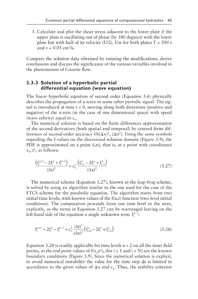
The numerical solution is based on the finite differences approximation
of the second derivatives (both spatial and temporal) by centred finite differences of second-order accuracy O((Δx) 2 , (Δt) 2 ). Using the same symbols
regarding the f values on the discretized solution domain (Figure 3.9), the
PDE is approximated on a point (i,n), that is, at a point with coordinates
x i , t n , as follows:
f
f
f
t
c
f
f
f
i
n
i
n
i
n
o
i
n
i
n
i
n
+
−
+
−
−
+
(
) =
−
+
(
)
1
1
2
2
1
1
2
2
( )
(
∆
∆ x x)
2
(3.27)
The numerical scheme (Equation 3.27), known as the leap-frog scheme,
is solved by using an algorithm similar to the one used for the case of the
FTCS scheme for the parabolic equation. The algorithm starts from two
initial time levels, with known values of the f(x,t) function (two-level initial
conditions). The computation proceeds from one time level to the next,
explicitly, as the terms in Equation 3.27 can be rearranged leaving on the
left-hand side of the equation a single unknown term f i
n+1
:
f
f f
c
t
x
f
f f
i
n
i
n
i
n
o
i
n
i
n
i
n
+
−
+
−
=
−
+
−
+
(
1
1
2
2
2
1
1
2
2
( )
( )
∆
∆
) )
(3.28)
Equation 3.28 is readily applicable for time levels n > 2 on all the inner field
points, as the end point values of f(x i ,t n ), (for i = 1 and i = N) are the known
boundary conditions (Figure 3.9). Since the numerical solution is explicit,
to avoid numerical instability the value for the time step Δt is limited in
accordance to the given values of Δx and c o . Thus, the stability criterion
5. Calculate and plot the shear stress adjacent to the lower plate if the
upper plate is oscillating out of phase (by 180 degrees) with the lower
plate but with half of its velocity (U/2). Use for both plates T = 500 s
and v = 0.05 cm 2 /s.
Compare the solution data obtained by running the modifications, derive
conclusions and discuss the significance of the various variables involved in
the phenomenon of Couette flow.
3.3.3 Solution of a hyperbolic partial
differential equation (wave equation)
The linear hyperbolic equation of second order (Equation 3.6) physically
describes the propagation of a wave or some other periodic signal. The signal is introduced at time t = 0, moving along both directions (positive and
negative) of the x-axis (in the case of one dimensional space) with speed
(wave celerity) equal to c o .
The numerical solution is based on the finite differences approximation
of the second derivatives (both spatial and temporal) by centred finite differences of second-order accuracy O((Δx) 2 , (Δt) 2 ). Using the same symbols
regarding the f values on the discretized solution domain (Figure 3.9), the
PDE is approximated on a point (i,n), that is, at a point with coordinates
x i , t n , as follows:
f
f
f
t
c
f
f
f
i
n
i
n
i
n
o
i
n
i
n
i
n
+
−
+
−
−
+
(
) =
−
+
(
)
1
1
2
2
1
1
2
2
( )
(
∆
∆ x x)
2
(3.27)
The numerical scheme (Equation 3.27), known as the leap-frog scheme,
is solved by using an algorithm similar to the one used for the case of the
FTCS scheme for the parabolic equation. The algorithm starts from two
initial time levels, with known values of the f(x,t) function (two-level initial
conditions). The computation proceeds from one time level to the next,
explicitly, as the terms in Equation 3.27 can be rearranged leaving on the
left-hand side of the equation a single unknown term f i
n+1
:
f
f f
c
t
x
f
f f
i
n
i
n
i
n
o
i
n
i
n
i
n
+
−
+
−
=
−
+
−
+
(
1
1
2
2
2
1
1
2
2
( )
( )
∆
∆
) )
(3.28)
Equation 3.28 is readily applicable for time levels n > 2 on all the inner field
points, as the end point values of f(x i ,t n ), (for i = 1 and i = N) are the known
boundary conditions (Figure 3.9). Since the numerical solution is explicit,
to avoid numerical instability the value for the time step Δt is limited in
accordance to the given values of Δx and c o . Thus, the stability criterion