

Ordinary differential equations 23
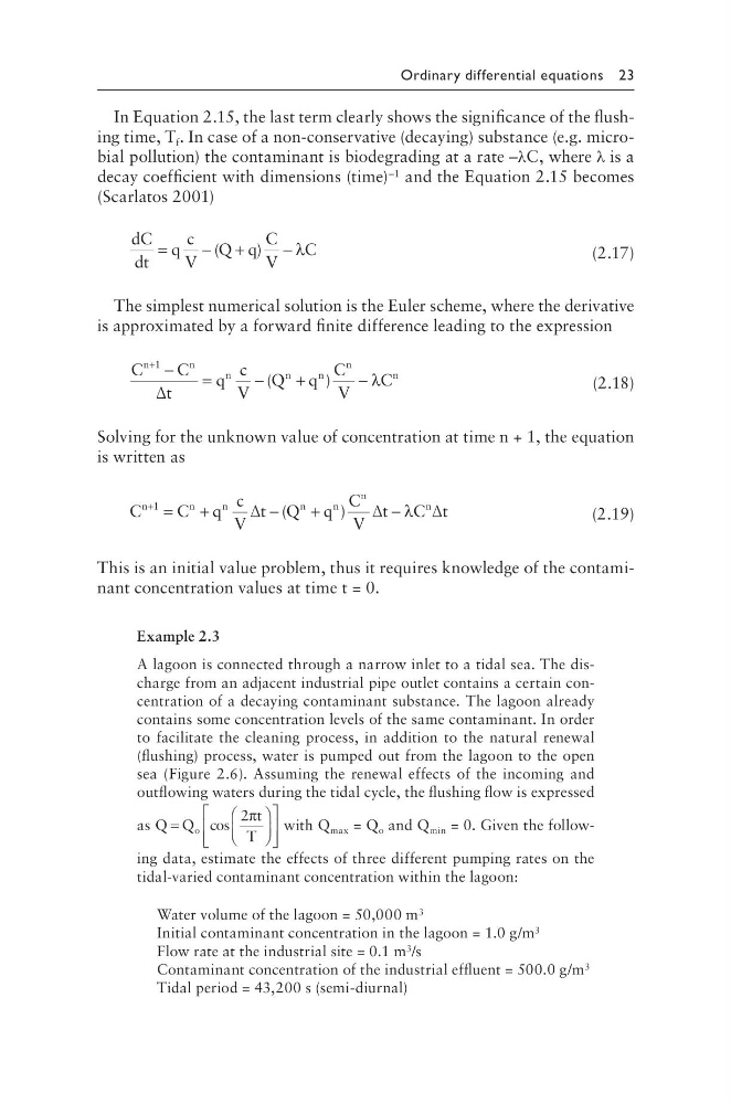
In Equation 2.15, the last term clearly shows the significance of the flushing time, T f . In case of a non-conservative (decaying) substance (e.g. microbial pollution) the contaminant is biodegrading at a rate –λC, where λ is a
decay coefficient with dimensions (time) –1 and the Equation 2.15 becomes
(Scarlatos 2001)
dC
dt
q
c
V
Q q
C
V
C
=
− +
−
(
)
λ
(2.17)
The simplest numerical solution is the Euler scheme, where the derivative
is approximated by a forward finite difference leading to the expression
C
C
t
q
c
V
Q q
C
V
C
n
n
n
n
n
n
n
+
−
=
−
+
−
1
∆
(
)
λ
(2.18)
Solving for the unknown value of concentration at time n + 1, the equation
is written as
C
C q
c
V
t Q q
C
V
t
C t
n
n
n
n
n
n
n
+
=
+
−
+
−
1
∆
∆
∆
(
)
λ
(2.19)
This is an initial value problem, thus it requires knowledge of the contaminant concentration values at time t = 0.
Example 2.3
A lagoon is connected through a narrow inlet to a tidal sea. The discharge from an adjacent industrial pipe outlet contains a certain concentration of a decaying contaminant substance. The lagoon already
contains some concentration levels of the same contaminant. In order
to facilitate the cleaning process, in addition to the natural renewal
(flushing) process, water is pumped out from the lagoon to the open
sea (Figure 2.6). Assuming the renewal effects of the incoming and
outflowing waters during the tidal cycle, the flushing flow is expressed
as Q Q
t
T
o
=
cos
2π
with Q max = Q o and Q min = 0. Given the following data, estimate the effects of three different pumping rates on the
tidal-varied contaminant concentration within the lagoon:
Water volume of the lagoon = 50,000 m 3
Initial contaminant concentration in the lagoon = 1.0 g/m 3
Flow rate at the industrial site = 0.1 m 3 /s
Contaminant concentration of the industrial effluent = 500.0 g/m 3
Tidal period = 43,200 s (semi-diurnal)
In Equation 2.15, the last term clearly shows the significance of the flushing time, T f . In case of a non-conservative (decaying) substance (e.g. microbial pollution) the contaminant is biodegrading at a rate –λC, where λ is a
decay coefficient with dimensions (time) –1 and the Equation 2.15 becomes
(Scarlatos 2001)
dC
dt
q
c
V
Q q
C
V
C
=
− +
−
(
)
λ
(2.17)
The simplest numerical solution is the Euler scheme, where the derivative
is approximated by a forward finite difference leading to the expression
C
C
t
q
c
V
Q q
C
V
C
n
n
n
n
n
n
n
+
−
=
−
+
−
1
∆
(
)
λ
(2.18)
Solving for the unknown value of concentration at time n + 1, the equation
is written as
C
C q
c
V
t Q q
C
V
t
C t
n
n
n
n
n
n
n
+
=
+
−
+
−
1
∆
∆
∆
(
)
λ
(2.19)
This is an initial value problem, thus it requires knowledge of the contaminant concentration values at time t = 0.
Example 2.3
A lagoon is connected through a narrow inlet to a tidal sea. The discharge from an adjacent industrial pipe outlet contains a certain concentration of a decaying contaminant substance. The lagoon already
contains some concentration levels of the same contaminant. In order
to facilitate the cleaning process, in addition to the natural renewal
(flushing) process, water is pumped out from the lagoon to the open
sea (Figure 2.6). Assuming the renewal effects of the incoming and
outflowing waters during the tidal cycle, the flushing flow is expressed
as Q Q
t
T
o
=
cos
2π
with Q max = Q o and Q min = 0. Given the following data, estimate the effects of three different pumping rates on the
tidal-varied contaminant concentration within the lagoon:
Water volume of the lagoon = 50,000 m 3
Initial contaminant concentration in the lagoon = 1.0 g/m 3
Flow rate at the industrial site = 0.1 m 3 /s
Contaminant concentration of the industrial effluent = 500.0 g/m 3
Tidal period = 43,200 s (semi-diurnal)