260 Computational Modelling in Hydraulic and Coastal Engineering
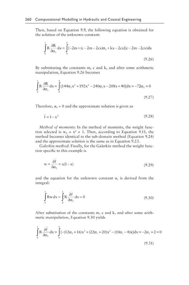
Then, based on Equation 9.9, the following equation is obtained for
the solution of the unknown constant:
R
R dx
m c m cx
kx cx c m cx
∂
∂
= −
+ −
−
+ −
−
−
∫ α
α
1
0
1
1
2
2
2
2
2
2
[
(
)
] (
) d dx
0
1
∫
(9.26)
By substituting the constants m, c and k, and after some arithmetic
manipulation, Equation 9.26 becomes
R
R dx
x
x
x
x
dx
∂
∂
=
+
−
−
+
=−
∫ α
α
α
1
0
1
1
2
2
1
144
192
240
208 40
7
[
]
2 2
0
1
0
1
α =
∫
(9.27)
Therefore, α 1 = 0 and the approximate solution is given as

f
x
= −
1
2
(9.28)
Method of moments: In the method of moments, the weight function selected is w 0 = x 0 = 1. Then, according to Equation 9.11, the
method becomes identical to the sub-domain method (Equation 9.24)
and the approximate solution is the same as in Equation 9.23.
Galerkin method: Finally, for the Galerkin method the weight function specific to this example is
w
f
x
x
=
∂
∂
=
−

α 1
1
(
)
(9.29)
and the equation for the unknown constant α 1 is derived from the
integral:
Rw dx
R
f dx
0
1
1
0
1
0
∫
∫
=
∂
∂
=

α
(9.30)
After substitution of the constants m, c and k, and after some arithmetic manipulation, Equation 9.30 yields
R
f dx
x
x
∂
∂
= −
+
+
+
−
−
∫

α
α
α
α
1
0
1
1
3
1
2
1
12
16
22
20
10
4
[ (
)
(
)
(
)x x dx
] = −
+ =
∫
2
2 0
1
0
1
α
(9.31)