

258 Computational Modelling in Hydraulic and Coastal Engineering
Normally, the accuracy of the approximated solution should improve
by increasing the order of the trial functions in Equation 9.2. However, an
increase in the number of the trial functions causes substantial complexity
on the required preliminary steps for the weighted residual methods.
Example 9.1
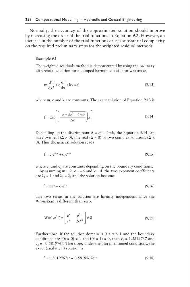
The weighted residuals method is demonstrated by using the ordinary
differential equation for a damped harmonic oscillator written as
m
d f
dx
c
df
dx
kx
2
2
0
+
+
=
(9.13)
where m, c and k are constants. The exact solution of Equation 9.13 is
f
c
c
mk
m
x
=
− ±
−
exp
2
4
2
(9.14)
Depending on the discriminant Δ = c 2 − 4mk, the Equation 9.14 can
have two real (Δ > 0), one real (Δ = 0) or two complex solutions (Δ <
0). Thus the general solution reads
f c e
c e
x
x
=
+
1
2
1
2
λ
λ
(9.15)
where c 1 and c 2 are constants depending on the boundary conditions.
By assuming m = 2, c = –6 and k = 4, the two exponent coefficients
are λ 1 = 1 and λ 2 = 2, and the solution becomes
f = c 1 e x + c 2 e 2x
(9.16)
The two terms in the solution are linearly independent since the
Wronskian is different than zero:
W e e
e
e
e
e
x
x
x
x
x
x
( , )
2
2
2
2
0
=
≠
(9.17)
Furthermore, if the solution domain is 0 ≤ x ≤ 1 and the boundary
conditions are f(x = 0) = 1 and f(x = 1) = 0, then c 1 = 1.5819767 and
c 2 = –0.5819767. Therefore, under the aforementioned conditions, the
exact (analytical) solution is
f = 1.5819767e x − 0.5819767e 2x
(9.18)
Normally, the accuracy of the approximated solution should improve
by increasing the order of the trial functions in Equation 9.2. However, an
increase in the number of the trial functions causes substantial complexity
on the required preliminary steps for the weighted residual methods.
Example 9.1
The weighted residuals method is demonstrated by using the ordinary
differential equation for a damped harmonic oscillator written as
m
d f
dx
c
df
dx
kx
2
2
0
+
+
=
(9.13)
where m, c and k are constants. The exact solution of Equation 9.13 is
f
c
c
mk
m
x
=
− ±
−
exp
2
4
2
(9.14)
Depending on the discriminant Δ = c 2 − 4mk, the Equation 9.14 can
have two real (Δ > 0), one real (Δ = 0) or two complex solutions (Δ <
0). Thus the general solution reads
f c e
c e
x
x
=
+
1
2
1
2
λ
λ
(9.15)
where c 1 and c 2 are constants depending on the boundary conditions.
By assuming m = 2, c = –6 and k = 4, the two exponent coefficients
are λ 1 = 1 and λ 2 = 2, and the solution becomes
f = c 1 e x + c 2 e 2x
(9.16)
The two terms in the solution are linearly independent since the
Wronskian is different than zero:
W e e
e
e
e
e
x
x
x
x
x
x
( , )
2
2
2
2
0
=
≠
(9.17)
Furthermore, if the solution domain is 0 ≤ x ≤ 1 and the boundary
conditions are f(x = 0) = 1 and f(x = 1) = 0, then c 1 = 1.5819767 and
c 2 = –0.5819767. Therefore, under the aforementioned conditions, the
exact (analytical) solution is
f = 1.5819767e x − 0.5819767e 2x
(9.18)