256 Computational Modelling in Hydraulic and Coastal Engineering
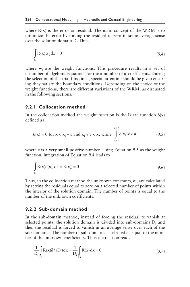
where R(x) is the error or residual. The main concept of the WRM is to
minimize the error by forcing the residual to zero in some average sense
over the solution domain D. Thus,
R x w dx
i
D
( )
∫
= 0
(9.4)
where w i are the weight functions. This procedure results in a set of
n- number of algebraic equations for the n-number of α i coefficients. During
the selection of the trial functions, special attention should be given ensuring they satisfy the boundary conditions. Depending on the choice of the
weight functions, there are different variations of the WRM, as discussed
in the following sections.
9.2.1 Collocation method
In the collocation method the weight function is the Dirac function δ(x)
defined as
δ(x) = 0 for x < x i – ε and x i + ε < x, while
δ
ε
ε
( )
x dx
i
x
x
i
i
=
−
+
∫
1
(9.5)
where ε is a very small positive number. Using Equation 9.5 as the weight
function, integration of Equation 9.4 leads to
R x x dx R x
i
D
i
( ) ( )
( )
δ
∫
=
=0
(9.6)
Thus, in the collocation method the unknown constants, α i , are calculated
by setting the residuals equal to zero on a selected number of points within
the interior of the solution domain. The number of points is equal to the
number of the unknown coefficients.
9.2.2 Sub-domain method
In the sub-domain method, instead of forcing the residual to vanish at
selected points, the solution domain is divided into sub-domains D i and
then the residual is forced to vanish in an average sense over each of the
sub-domains. The number of sub-domains is selected as equal to the number of the unknown coefficients. Thus the relation reads
1
1
0
D
R x
D dx D
R x dx
i
i
D
i D
i
i
( ) *( )
()
δ
∫
∫
=
=
(9.7)