202 Computational Modelling in Hydraulic and Coastal Engineering
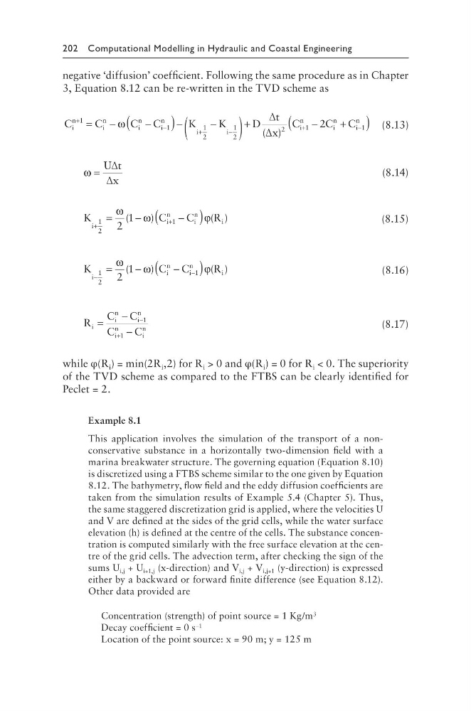
negative ‘diffusion’ coefficient. Following the same procedure as in Chapter
3, Equation 8.12 can be re-written in the TVD scheme as
C
C
C C
K
K
D
t
x
C
i
n
i
n
i
n
i
n
i
i
i
+
−
+
−
=
−
−
(
)−
−
(
)
+
1
1
1
2
1
2
2
ω
∆
∆
( )
+ +
−
−
+
(
)
1
1
2
n
i
n
i
n
C C
(8.13)
ω =
U t
x
∆
∆
(8.14)
K
C
C
R
i
i
n
i
n
i
+
+
=
−
−
(
)
1
2
1
2
1
ω
ω
ϕ
(
)
( )
(8.15)
K
C C
R
i
i
n
i
n
i
−
−
=
−
−
(
)
1
2
1
2
1
ω
ω
ϕ
(
)
( )
(8.16)
R
C C
C
C
i
i
n
i
n
i
n
i
n
=
−
−
−
+
1
1
(8.17)
while φ(R i ) = min(2R i ,2) for R i > 0 and φ(R i ) = 0 for R i < 0. The superiority
of the TVD scheme as compared to the FTBS can be clearly identified for
Peclet = 2.
Example 8.1
This application involves the simulation of the transport of a nonconservative substance in a horizontally two-dimension field with a
marina breakwater structure. The governing equation (Equation 8.10)
is discretized using a FTBS scheme similar to the one given by Equation
8.12. The bathymetry, flow field and the eddy diffusion coefficients are
taken from the simulation results of Example 5.4 (Chapter 5). Thus,
the same staggered discretization grid is applied, where the velocities U
and V are defined at the sides of the grid cells, while the water surface
elevation (h) is defined at the centre of the cells. The substance concentration is computed similarly with the free surface elevation at the centre of the grid cells. The advection term, after checking the sign of the
sums U i,j + U i+1,j (x-direction) and V i,j + V i,j+1 (y-direction) is expressed
either by a backward or forward finite difference (see Equation 8.12).
Other data provided are
Concentration (strength) of point source = 1 Kg/m 3
Decay coefficient = 0 s –1
Location of the point source: x = 90 m; y = 125 m