200 Computational Modelling in Hydraulic and Coastal Engineering
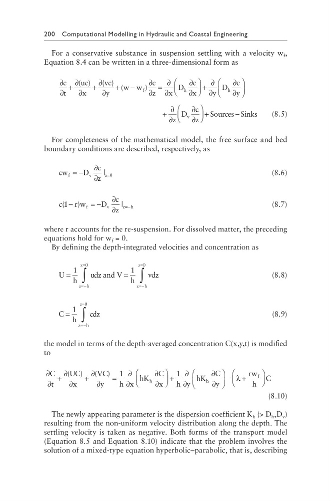
For a conservative substance in suspension settling with a velocity w f ,
Equation 8.4 can be written in a three-dimensional form as
∂
∂
+
∂
∂
+
∂
∂
+ −
∂
∂
=
∂
∂
∂
∂

 

 
c
t
uc
x
vc
y
w w
c
z
x
D
c
x
f
h
( )
( ) (
)
+ +
∂
∂
∂
∂

 

 
+
∂
∂
∂
∂

 

  +
−
y
D
c
y
z
D
c
z
Sources Sinks
h
v
(8.5)
For completeness of the mathematical model, the free surface and bed
boundary conditions are described, respectively, as
cw
D
c
z
f
v
z
= −
∂
∂
=
| 0
(8.6)
c
r w
D
c
z
f
v
z h
(
)
|
1 −
=−
∂
∂
=−
(8.7)
where r accounts for the re-suspension. For dissolved matter, the preceding
equations hold for w f = 0.
By defining the depth-integrated velocities and concentration as
U h
udz and V h
vdz
z h
z
z h
z
=
=
=−
=
=−
=
∫
∫
1
1
0
0
(8.8)
C h
cdz
z h
z
=
=−
=
∫
1
0
(8.9)
the model in terms of the depth-averaged concentration C(x,y,t) is modified
to
∂
∂
+
∂
∂
+
∂
∂
=
∂
∂
∂
∂

 

  +
∂
∂
C
t
UC
x
VC
y
h x
hK
C
x
h y
hK
h
( )
( ) 1
1
h h
f
C
y
rw
h
C
∂
∂

 

  −
+

 

 
λ
(8.10)
The newly appearing parameter is the dispersion coefficient K h (> D h ,D v )
resulting from the non-uniform velocity distribution along the depth. The
settling velocity is taken as negative. Both forms of the transport model
(Equation 8.5 and Equation 8.10) indicate that the problem involves the
solution of a mixed-type equation hyperbolic–parabolic, that is, describing