

Flow in porous media 179
aquifer. That delays the establishment of the equilibrium conditions
where water enters the aquifer from the ground upstream of the dam
and exits from the ground downstream of the dam.
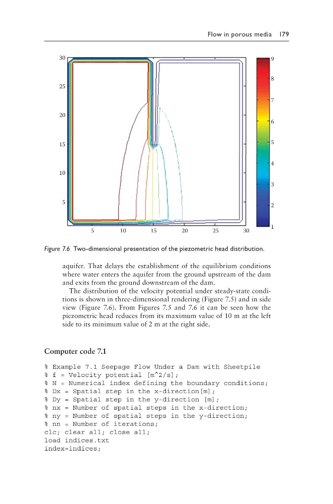
The distribution of the velocity potential under steady-state conditions is shown in three-dimensional rendering (Figure 7.5) and in side
view (Figure 7.6). From Figures 7.5 and 7.6 it can be seen how the
piezometric head reduces from its maximum value of 10 m at the left
side to its minimum value of 2 m at the right side.
Computer code 7.1
% Example 7.1 Seepage Flow Under a Dam with Sheetpile
% f = Velocity potential [m^2/s];
% N = Numerical index defining the boundary conditions;
% Dx = Spatial step in the x-direction[m];
% Dy = Spatial step in the y-direction [m];
% nx = Number of spatial steps in the x-direction;
% ny = Number of spatial steps in the y-direction;
% nn = Number of iterations;
clc; clear all; close all;
load indices.txt
index=indices;
30
25
20
15
10
5
5
1 0
1 5
2 0
2 5
3 0
9
8
7
6
5
4
3
2
1
Figure 7.6 Two-dimensional presentation of the piezometric head distribution.
aquifer. That delays the establishment of the equilibrium conditions
where water enters the aquifer from the ground upstream of the dam
and exits from the ground downstream of the dam.
The distribution of the velocity potential under steady-state conditions is shown in three-dimensional rendering (Figure 7.5) and in side
view (Figure 7.6). From Figures 7.5 and 7.6 it can be seen how the
piezometric head reduces from its maximum value of 10 m at the left
side to its minimum value of 2 m at the right side.
Computer code 7.1
% Example 7.1 Seepage Flow Under a Dam with Sheetpile
% f = Velocity potential [m^2/s];
% N = Numerical index defining the boundary conditions;
% Dx = Spatial step in the x-direction[m];
% Dy = Spatial step in the y-direction [m];
% nx = Number of spatial steps in the x-direction;
% ny = Number of spatial steps in the y-direction;
% nn = Number of iterations;
clc; clear all; close all;
load indices.txt
index=indices;
30
25
20
15
10
5
5
1 0
1 5
2 0
2 5
3 0
9
8
7
6
5
4
3
2
1
Figure 7.6 Two-dimensional presentation of the piezometric head distribution.