

Surface gravity water waves 165
The variability of all 40 Fourier series coefficients α k and β k at the
mid-point of the basin is depicted in Figure 6.11.
Finally, from the periodogram, that is, plot of the amplitude
α β
k
k
2
2
+
versus the wave number k (= 1 to 40) of the Fourier series
components (Figure 6.12), the corresponding k j wave numbers are
identified and the periods of natural oscillations are estimated according to Equation 6.28. The natural oscillation periods estimated by the
Fourier series analysis and by the Merian formula (Equation 6.29) are
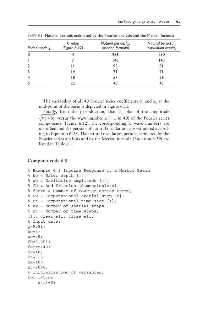
listed in Table 6.1.
Computer code 6.5
% Example 6.5 Impulse Response of a Harbor Basin
% ho = Water depth [m];
% zo = Excitation amplitude [m];
% fb = Bed friction [dimensionless];
% fsero = Number of Fourier series terms;
% Dx = Computational spatial step [m];
% Dt = Computational time step [s];
% nx = Number of spatial steps;
% nt = Number of time steps;
clc; clear all; close all;
% Input data;
g=9.81;
ho=5;
zo=.5;
fb=0.001;
fsero=40;
Dx=10;
Dt=0.5;
nx=100;
nt=2000;
% Initialization of variables;
for i=1:nx
z(i)=0;
Table 6.1 Natural periods estimated by the Fourier analysis and the Merian formula
Period mode, j
k j value
(Figure 6.12)
Natural period, T jM
(Merian formula)
Natural period, T jS
(simulation results)
0
4
286
250
1
7
143
143
2
11
95
91
3
14
71
71
4
18
57
56
5
22
48
45
The variability of all 40 Fourier series coefficients α k and β k at the
mid-point of the basin is depicted in Figure 6.11.
Finally, from the periodogram, that is, plot of the amplitude
α β
k
k
2
2
+
versus the wave number k (= 1 to 40) of the Fourier series
components (Figure 6.12), the corresponding k j wave numbers are
identified and the periods of natural oscillations are estimated according to Equation 6.28. The natural oscillation periods estimated by the
Fourier series analysis and by the Merian formula (Equation 6.29) are
listed in Table 6.1.
Computer code 6.5
% Example 6.5 Impulse Response of a Harbor Basin
% ho = Water depth [m];
% zo = Excitation amplitude [m];
% fb = Bed friction [dimensionless];
% fsero = Number of Fourier series terms;
% Dx = Computational spatial step [m];
% Dt = Computational time step [s];
% nx = Number of spatial steps;
% nt = Number of time steps;
clc; clear all; close all;
% Input data;
g=9.81;
ho=5;
zo=.5;
fb=0.001;
fsero=40;
Dx=10;
Dt=0.5;
nx=100;
nt=2000;
% Initialization of variables;
for i=1:nx
z(i)=0;
Table 6.1 Natural periods estimated by the Fourier analysis and the Merian formula
Period mode, j
k j value
(Figure 6.12)
Natural period, T jM
(Merian formula)
Natural period, T jS
(simulation results)
0
4
286
250
1
7
143
143
2
11
95
91
3
14
71
71
4
18
57
56
5
22
48
45