

Surface gravity water waves 153
The preceding equations can be solved numerically by using a centred
second-order finite differences scheme for both time and space derivatives.
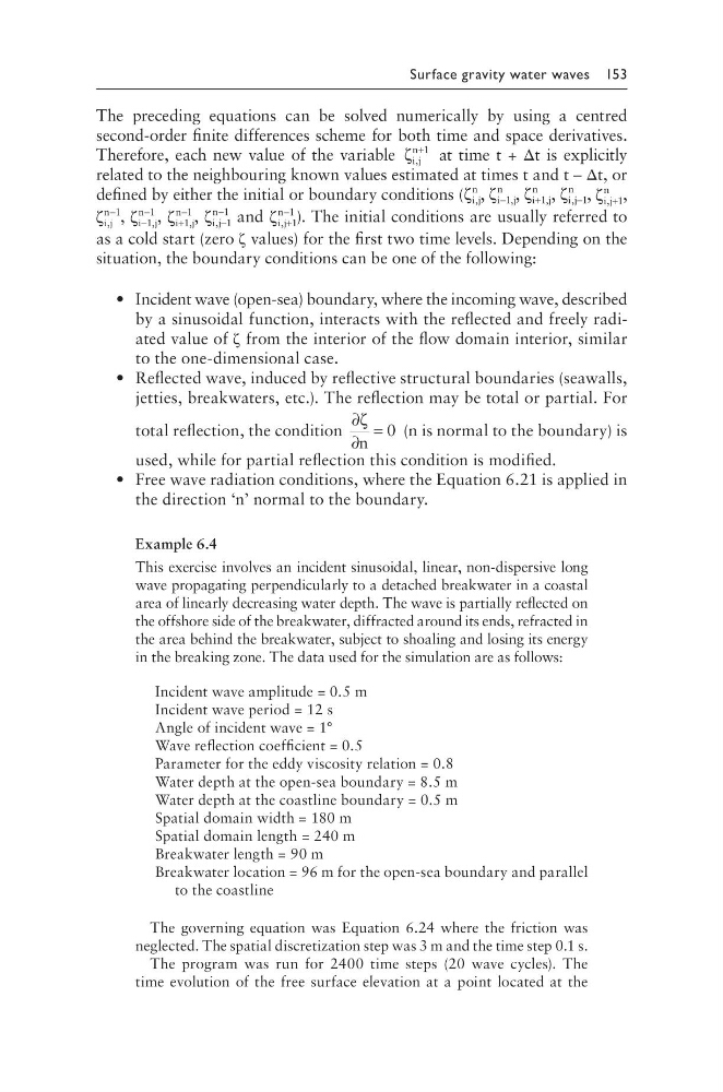
Therefore, each new value of the variable ζ i j
n
,
+1
at time t + Δt is explicitly
related to the neighbouring known values estimated at times t and t – Δt, or
defined by either the initial or boundary conditions (ζ i j
n
, , ζ i j
n
−1, , ζ i j
n
+1, , ζ i j
n
, −1 , ζ i j
n
, +1 ,
ζ i j
n
,
−1
, ζ i j
n
−
−
1
1
, , ζ i j
n
+
−
1
1
, , ζ i j
n
, −
−
1
1
and ζ i j
n
, +
−
1
1
). The initial conditions are usually referred to
as a cold start (zero ζ values) for the first two time levels. Depending on the
situation, the boundary conditions can be one of the following:
• Incident wave (open-sea) boundary, where the incoming wave, described
by a sinusoidal function, interacts with the reflected and freely radiated value of ζ from the interior of the flow domain interior, similar
to the one-dimensional case.
• Reflected wave, induced by reflective structural boundaries (seawalls,
jetties, breakwaters, etc.). The reflection may be total or partial. For
total reflection, the condition
∂
∂
=
ζ
n
0 (n is normal to the boundary) is
used, while for partial reflection this condition is modified.
• Free wave radiation conditions, where the Equation 6.21 is applied in
the direction ‘n’ normal to the boundary.
Example 6.4
This exercise involves an incident sinusoidal, linear, non-dispersive long
wave propagating perpendicularly to a detached breakwater in a coastal
area of linearly decreasing water depth. The wave is partially reflected on
the offshore side of the breakwater, diffracted around its ends, refracted in
the area behind the breakwater, subject to shoaling and losing its energy
in the breaking zone. The data used for the simulation are as follows:
Incident wave amplitude = 0.5 m
Incident wave period = 12 s
Angle of incident wave = 1°
Wave reflection coefficient = 0.5
Parameter for the eddy viscosity relation = 0.8
Water depth at the open-sea boundary = 8.5 m
Water depth at the coastline boundary = 0.5 m
Spatial domain width = 180 m
Spatial domain length = 240 m
Breakwater length = 90 m
Breakwater location = 96 m for the open-sea boundary and parallel
to the coastline
The governing equation was Equation 6.24 where the friction was
neglected. The spatial discretization step was 3 m and the time step 0.1 s.
The program was run for 2400 time steps (20 wave cycles). The
time evolution of the free surface elevation at a point located at the
The preceding equations can be solved numerically by using a centred
second-order finite differences scheme for both time and space derivatives.
Therefore, each new value of the variable ζ i j
n
,
+1
at time t + Δt is explicitly
related to the neighbouring known values estimated at times t and t – Δt, or
defined by either the initial or boundary conditions (ζ i j
n
, , ζ i j
n
−1, , ζ i j
n
+1, , ζ i j
n
, −1 , ζ i j
n
, +1 ,
ζ i j
n
,
−1
, ζ i j
n
−
−
1
1
, , ζ i j
n
+
−
1
1
, , ζ i j
n
, −
−
1
1
and ζ i j
n
, +
−
1
1
). The initial conditions are usually referred to
as a cold start (zero ζ values) for the first two time levels. Depending on the
situation, the boundary conditions can be one of the following:
• Incident wave (open-sea) boundary, where the incoming wave, described
by a sinusoidal function, interacts with the reflected and freely radiated value of ζ from the interior of the flow domain interior, similar
to the one-dimensional case.
• Reflected wave, induced by reflective structural boundaries (seawalls,
jetties, breakwaters, etc.). The reflection may be total or partial. For
total reflection, the condition
∂
∂
=
ζ
n
0 (n is normal to the boundary) is
used, while for partial reflection this condition is modified.
• Free wave radiation conditions, where the Equation 6.21 is applied in
the direction ‘n’ normal to the boundary.
Example 6.4
This exercise involves an incident sinusoidal, linear, non-dispersive long
wave propagating perpendicularly to a detached breakwater in a coastal
area of linearly decreasing water depth. The wave is partially reflected on
the offshore side of the breakwater, diffracted around its ends, refracted in
the area behind the breakwater, subject to shoaling and losing its energy
in the breaking zone. The data used for the simulation are as follows:
Incident wave amplitude = 0.5 m
Incident wave period = 12 s
Angle of incident wave = 1°
Wave reflection coefficient = 0.5
Parameter for the eddy viscosity relation = 0.8
Water depth at the open-sea boundary = 8.5 m
Water depth at the coastline boundary = 0.5 m
Spatial domain width = 180 m
Spatial domain length = 240 m
Breakwater length = 90 m
Breakwater location = 96 m for the open-sea boundary and parallel
to the coastline
The governing equation was Equation 6.24 where the friction was
neglected. The spatial discretization step was 3 m and the time step 0.1 s.
The program was run for 2400 time steps (20 wave cycles). The
time evolution of the free surface elevation at a point located at the