

Introduction 3
Also, for a mathematical model to be well-posed, it is necessary that the
governing PDEs, the auxiliary data and the numerical algorithm are all
well-posed.
1.1.1.2 Discretization and numerical solution
of mathematical models
In numerical models the governing equations are reformulated in approximate manner, like when the differential equations are written as difference
equations, by means of some numerical method. The solution domain is
also appropriately discretized into one-, two- or three-dimensional cells,
and the solution is approximated on the corner nodes, sides or the interior
of the cells. Discretization of the continuous independent variables x, y, z
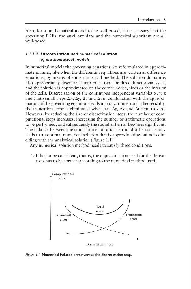
and t into small steps Δx, Δy, Δz and Δt in combination with the approximation of the governing equations leads to truncation errors. Theoretically,
the truncation error is eliminated when Δx, Δy, Δz and Δt tend to zero.
However, by reducing the size of discretization steps, the number of computational steps increases, increasing the number or arithmetic operations
to be performed, and subsequently the round-off error becomes significant.
The balance between the truncation error and the round-off error usually
leads to an optimal numerical solution that is approximating but not coinciding with the analytical solution (Figure 1.1).
Any numerical solution method needs to satisfy three conditions:
1. It has to be consistent, that is, the approximation used for the derivatives has to be correct, according to the numerical method used.
Total
error
Computational
error
Truncation
error
Round-off
error
Discretization step
Figure 1.1 Numerical induced error versus the discretization step.
Also, for a mathematical model to be well-posed, it is necessary that the
governing PDEs, the auxiliary data and the numerical algorithm are all
well-posed.
1.1.1.2 Discretization and numerical solution
of mathematical models
In numerical models the governing equations are reformulated in approximate manner, like when the differential equations are written as difference
equations, by means of some numerical method. The solution domain is
also appropriately discretized into one-, two- or three-dimensional cells,
and the solution is approximated on the corner nodes, sides or the interior
of the cells. Discretization of the continuous independent variables x, y, z
and t into small steps Δx, Δy, Δz and Δt in combination with the approximation of the governing equations leads to truncation errors. Theoretically,
the truncation error is eliminated when Δx, Δy, Δz and Δt tend to zero.
However, by reducing the size of discretization steps, the number of computational steps increases, increasing the number or arithmetic operations
to be performed, and subsequently the round-off error becomes significant.
The balance between the truncation error and the round-off error usually
leads to an optimal numerical solution that is approximating but not coinciding with the analytical solution (Figure 1.1).
Any numerical solution method needs to satisfy three conditions:
1. It has to be consistent, that is, the approximation used for the derivatives has to be correct, according to the numerical method used.
Total
error
Computational
error
Truncation
error
Round-off
error
Discretization step
Figure 1.1 Numerical induced error versus the discretization step.