

112 Computational Modelling in Hydraulic and Coastal Engineering
rectangular grid. The incoming from the left longshore current has
a constant velocity of 0.2 m/s. The right boundary is described by a
radiation (free-outflow) condition. The same free-outflow condition is
applied to the open-sea boundary condition. The input data used for
the simulation are as follows:
Water depth = 4 m
Smagorinsky parameter = 0.3
Coriolis coefficient = 0.0001 s –1
Bed friction = 0.001
The shape of the structure is provided in the text file (depths.txt).
The grid cells occupied by the coastline and the breakwater structure
are defined as zero depth, and the rest of the cells as 4 (indicative of the
water depth). The spatial discretization steps were Δx = Δy = 5 m and
the time step Δt = 0.5 s.
The computations started with a cold start where velocities and water
surface fluctuations were taken as zeros. The simulation was conducted
for 14,400 time steps (2.0 hours), since before that time the system
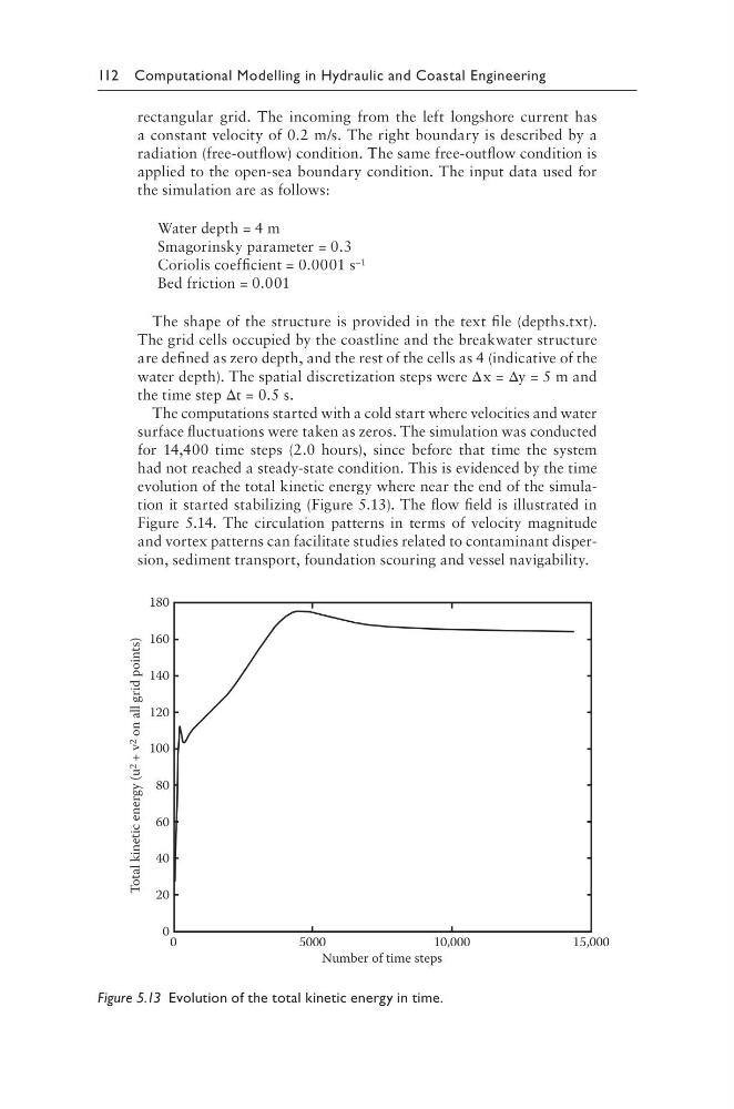
had not reached a steady-state condition. This is evidenced by the time
evolution of the total kinetic energy where near the end of the simulation it started stabilizing (Figure 5.13). The flow field is illustrated in
Figure 5.14. The circulation patterns in terms of velocity magnitude
and vortex patterns can facilitate studies related to contaminant dispersion, sediment transport, foundation scouring and vessel navigability.
180
160
140
120
100
80
60
40
20
0 0
5000
1 0,000
15,000
Number of time steps
Total kinetic energy (u 2
+ v 2
on all grid points)
Figure 5.13 Evolution of the total kinetic energy in time.
rectangular grid. The incoming from the left longshore current has
a constant velocity of 0.2 m/s. The right boundary is described by a
radiation (free-outflow) condition. The same free-outflow condition is
applied to the open-sea boundary condition. The input data used for
the simulation are as follows:
Water depth = 4 m
Smagorinsky parameter = 0.3
Coriolis coefficient = 0.0001 s –1
Bed friction = 0.001
The shape of the structure is provided in the text file (depths.txt).
The grid cells occupied by the coastline and the breakwater structure
are defined as zero depth, and the rest of the cells as 4 (indicative of the
water depth). The spatial discretization steps were Δx = Δy = 5 m and
the time step Δt = 0.5 s.
The computations started with a cold start where velocities and water
surface fluctuations were taken as zeros. The simulation was conducted
for 14,400 time steps (2.0 hours), since before that time the system
had not reached a steady-state condition. This is evidenced by the time
evolution of the total kinetic energy where near the end of the simulation it started stabilizing (Figure 5.13). The flow field is illustrated in
Figure 5.14. The circulation patterns in terms of velocity magnitude
and vortex patterns can facilitate studies related to contaminant dispersion, sediment transport, foundation scouring and vessel navigability.
180
160
140
120
100
80
60
40
20
0 0
5000
1 0,000
15,000
Number of time steps
Total kinetic energy (u 2
+ v 2
on all grid points)
Figure 5.13 Evolution of the total kinetic energy in time.