

110 Computational Modelling in Hydraulic and Coastal Engineering
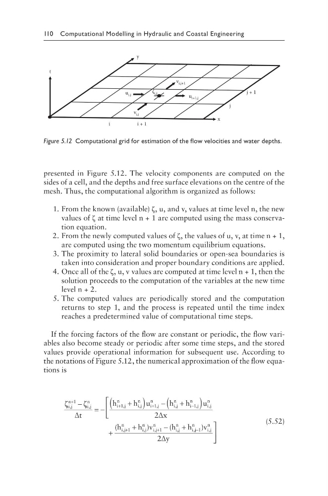
presented in Figure 5.12. The velocity components are computed on the
sides of a cell, and the depths and free surface elevations on the centre of the
mesh. Thus, the computational algorithm is organized as follows:
1. From the known (available) ζ, u, and v, values at time level n, the new
values of ζ at time level n + 1 are computed using the mass conservation equation.
2. From the newly computed values of ζ, the values of u, v, at time n + 1,
are computed using the two momentum equilibrium equations.
3. The proximity to lateral solid boundaries or open-sea boundaries is
taken into consideration and proper boundary conditions are applied.
4. Once all of the ζ, u, v values are computed at time level n + 1, then the
solution proceeds to the computation of the variables at the new time
level n + 2.
5. The computed values are periodically stored and the computation
returns to step 1, and the process is repeated until the time index
reaches a predetermined value of computational time steps.
If the forcing factors of the flow are constant or periodic, the flow variables also become steady or periodic after some time steps, and the stored
values provide operational information for subsequent use. According to
the notations of Figure 5.12, the numerical approximation of the flow equations is
ζ
ζ
i j
n
i j
n
i j
n
i j
n
i j
n
i j
n
t
h
h u
h
h
,
,
,
,
,
,
+
+
+
−
= −
+
(
) − +
1
1
1
∆
i i j
n
i j
n
i j
n
i j
n
i j
n
i
u
x
h
h v
h
−
+
+
(
)
+
+
−
1
1
1
2
,
,
,
,
,
(
)
(
∆
, ,
,
,
)
j
n
i j
n
i j
n
h
v
y
+
−1
2∆
(5.52)
j + 1
j
i + 1
u i+1,j
u i,j
v i,j
ζ i,j
i
v i,j+1
t
y
x
Figure 5.12 Computational grid for estimation of the flow velocities and water depths.
presented in Figure 5.12. The velocity components are computed on the
sides of a cell, and the depths and free surface elevations on the centre of the
mesh. Thus, the computational algorithm is organized as follows:
1. From the known (available) ζ, u, and v, values at time level n, the new
values of ζ at time level n + 1 are computed using the mass conservation equation.
2. From the newly computed values of ζ, the values of u, v, at time n + 1,
are computed using the two momentum equilibrium equations.
3. The proximity to lateral solid boundaries or open-sea boundaries is
taken into consideration and proper boundary conditions are applied.
4. Once all of the ζ, u, v values are computed at time level n + 1, then the
solution proceeds to the computation of the variables at the new time
level n + 2.
5. The computed values are periodically stored and the computation
returns to step 1, and the process is repeated until the time index
reaches a predetermined value of computational time steps.
If the forcing factors of the flow are constant or periodic, the flow variables also become steady or periodic after some time steps, and the stored
values provide operational information for subsequent use. According to
the notations of Figure 5.12, the numerical approximation of the flow equations is
ζ
ζ
i j
n
i j
n
i j
n
i j
n
i j
n
i j
n
t
h
h u
h
h
,
,
,
,
,
,
+
+
+
−
= −
+
(
) − +
1
1
1
∆
i i j
n
i j
n
i j
n
i j
n
i j
n
i
u
x
h
h v
h
−
+
+
(
)
+
+
−
1
1
1
2
,
,
,
,
,
(
)
(
∆
, ,
,
,
)
j
n
i j
n
i j
n
h
v
y
+
−1
2∆
(5.52)
j + 1
j
i + 1
u i+1,j
u i,j
v i,j
ζ i,j
i
v i,j+1
t
y
x
Figure 5.12 Computational grid for estimation of the flow velocities and water depths.