

STRUCTURAL MASS, DAMPING, AND RESTRAINT
45
The catenary is the curve formed by suspending a uniform cable of zéro
bending stiffness between two points. Classical theory for the static catenary
shape forms the basis for an upper bound calculation on the restraint stiffness
for cablestayed offshore structures. In this theory, longitudinal cable extension
is neglected, as are the effects of cable dynamics. Consider the cable segment of
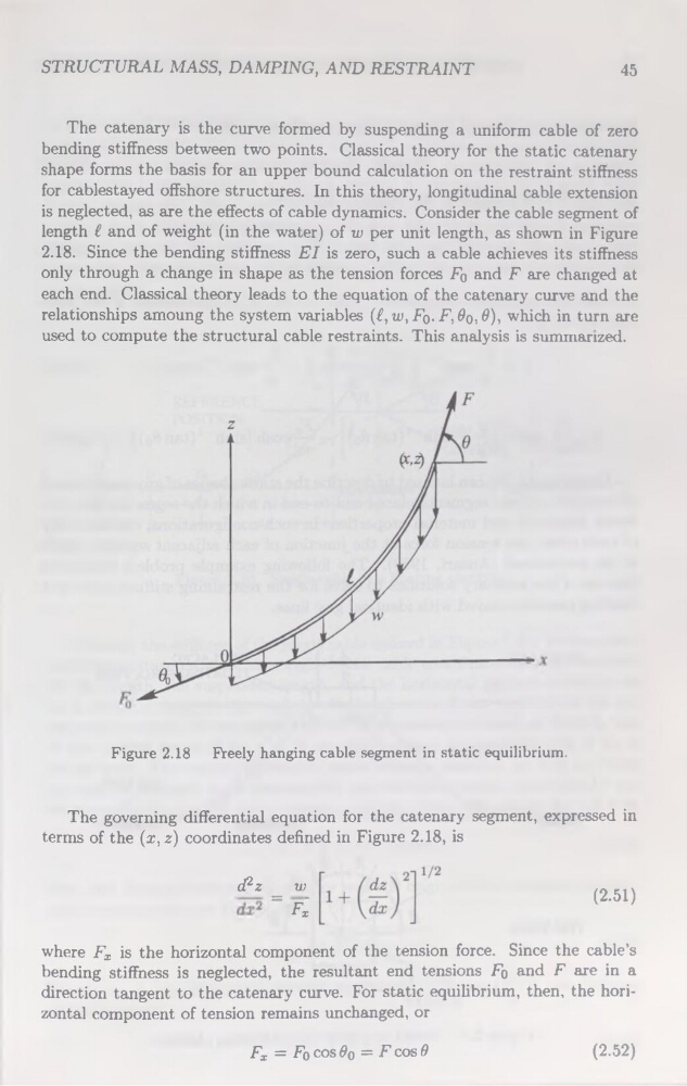
length £ and of weight (in the water) of w per unit length, as shown in Figure
2.18. Since the bending stiffness El is zéro, such a cable achieves its stiffness
only through a change in shape as the tension forces Fo and F are changed at
each end. Classical theory leads to the équation of the catenary curve and the
relationships amoung the System variables (£, w, Fq. F, Ôq, 6), which in turn are
used to compute the structural cable restraints. This analysis is summanzed.
Figure 2.18 Freely hanging cable segment in static equilibrium.
The governing differential équation for the catenary segment, expressed in
terms of the (x, z) coordinates defined in Figure 2.18, is
cPz
w
= F~x
(2.51)
where Fx is the horizontal component of the tension force. Since the cable’s
bending stiffness is neglected, the résultant end tensions Fq and F are in a
direction tangent to the catenary curve. For static equilibrium, then, the horizontal component of tension remains unchanged, or
Fx = Fo cos 0O = F cos 0
(2.52)
45
The catenary is the curve formed by suspending a uniform cable of zéro
bending stiffness between two points. Classical theory for the static catenary
shape forms the basis for an upper bound calculation on the restraint stiffness
for cablestayed offshore structures. In this theory, longitudinal cable extension
is neglected, as are the effects of cable dynamics. Consider the cable segment of
length £ and of weight (in the water) of w per unit length, as shown in Figure
2.18. Since the bending stiffness El is zéro, such a cable achieves its stiffness
only through a change in shape as the tension forces Fo and F are changed at
each end. Classical theory leads to the équation of the catenary curve and the
relationships amoung the System variables (£, w, Fq. F, Ôq, 6), which in turn are
used to compute the structural cable restraints. This analysis is summanzed.
Figure 2.18 Freely hanging cable segment in static equilibrium.
The governing differential équation for the catenary segment, expressed in
terms of the (x, z) coordinates defined in Figure 2.18, is
cPz
w
= F~x
(2.51)
where Fx is the horizontal component of the tension force. Since the cable’s
bending stiffness is neglected, the résultant end tensions Fq and F are in a
direction tangent to the catenary curve. For static equilibrium, then, the horizontal component of tension remains unchanged, or
Fx = Fo cos 0O = F cos 0
(2.52)