

280
CONTINUOUS SYSTEMS
Table 10.2 Typical Parameters for an OTEC System
Symbol
Meaning
Numerical Value
A
Wave spectrum amplitude
0.780 m’ 2 ■ (s/rad)6
B
Wave spectrum constant
0.0311 (rad/s)4
B0
Barge length
122 m
C
Barge frequency parameter
5.55 m1/2-rad/s
CA
Added mass coefficient
1.0
Cm
Inertia coefficient
2.0
d
Water depth
1067 m
D
Outside pipe diameter
9.144 m
ei
Sway frequency scale factor
0.093
«2
Sway amplitude scale factor
0.05
E
Young’s modulus for pipe
2.07x10“ N/m2
El
bending stiffness for pipe
3.94x10“ N-m2
9
Accélération due to gravity
9.81 m/s2
K
Rotational spring constant
1.13xl08 N-m/rad
L
Pipeline length
61 m to 1037 m
Mo
Ballast mass
4.54xl04 kg;
2.27 xlO5 kg
Mi
Ballast mass in water
O.6Mo
m
Pipe mass/unit length, incl. contents
6.43xl04 kg/m
771]
Pipe mass/unit length in water
1.25xlO3 kg/m
N
Number of waves in spectrum
15
P
Mass density of water
962 kg/m3
uq
Spectrum frequency, lower bound
0.1 rad/s
Ub
Sway weighting frequency
0.503 rad/s
un
Spectrum frequency, upper bound
1.5 rad/s
“p
Frequency at peak of Sn(w)
0.4 rad/s
Numerical Results
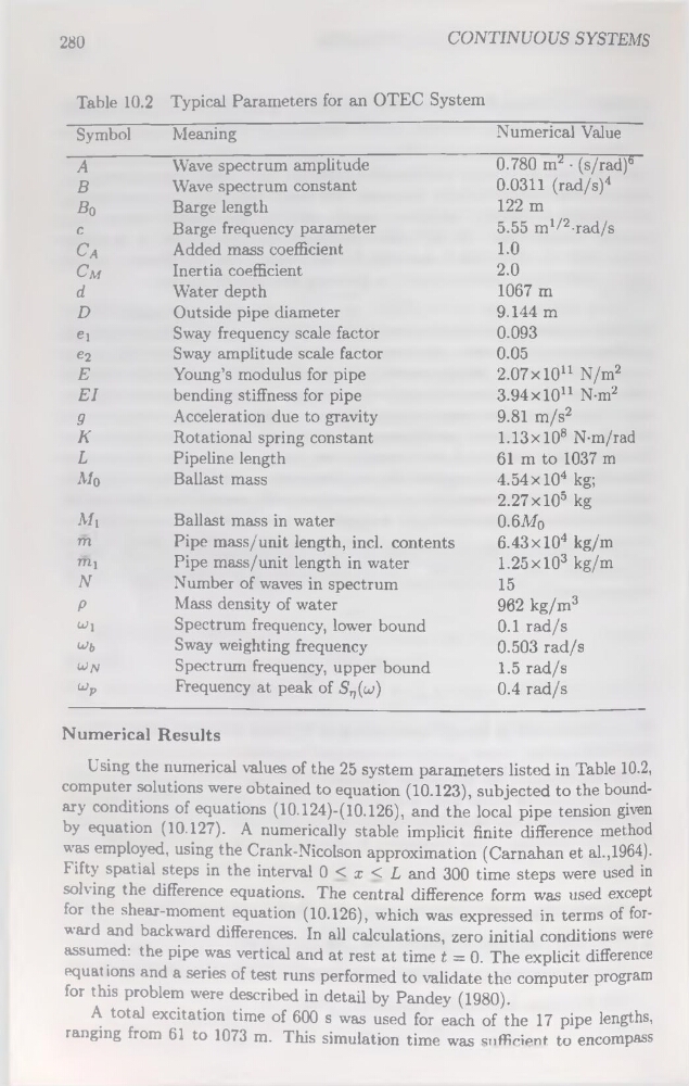
Using the numerical values of the 25 System parameters listed in Table 10.2,
computer solutions were obtained to équation (10.123), subjected to the boundary conditions of équations ( 10.124)-(10.126), and the local pipe tension given
by équation (10.127). A numerically stable implicit finite différence method
was employed, using the Crank-Nicolson approximation (Carnahan et al.,1964).
Fifty spatial steps in the interval 0 < x < L and 300 time steps were used in
solving the différence équations. The central différence form was used except
for the shear-moment équation (10.126), which was expressed in terms of forward and backward différences. In ail calculations, zéro initial conditions were
assumed: the pipe was vertical and at rest at time t = 0. The explicit différence
equat ions and a sériés of test runs performed to validate the computer program
for this problem were described in detail by Pandey (1980).
A total excitation time of 600 s was used for each of the 17 pipe lengths,
ranging from 61 to 1073 m. This simulation time was sufficient to encompass
CONTINUOUS SYSTEMS
Table 10.2 Typical Parameters for an OTEC System
Symbol
Meaning
Numerical Value
A
Wave spectrum amplitude
0.780 m’ 2 ■ (s/rad)6
B
Wave spectrum constant
0.0311 (rad/s)4
B0
Barge length
122 m
C
Barge frequency parameter
5.55 m1/2-rad/s
CA
Added mass coefficient
1.0
Cm
Inertia coefficient
2.0
d
Water depth
1067 m
D
Outside pipe diameter
9.144 m
ei
Sway frequency scale factor
0.093
«2
Sway amplitude scale factor
0.05
E
Young’s modulus for pipe
2.07x10“ N/m2
El
bending stiffness for pipe
3.94x10“ N-m2
9
Accélération due to gravity
9.81 m/s2
K
Rotational spring constant
1.13xl08 N-m/rad
L
Pipeline length
61 m to 1037 m
Mo
Ballast mass
4.54xl04 kg;
2.27 xlO5 kg
Mi
Ballast mass in water
O.6Mo
m
Pipe mass/unit length, incl. contents
6.43xl04 kg/m
771]
Pipe mass/unit length in water
1.25xlO3 kg/m
N
Number of waves in spectrum
15
P
Mass density of water
962 kg/m3
uq
Spectrum frequency, lower bound
0.1 rad/s
Ub
Sway weighting frequency
0.503 rad/s
un
Spectrum frequency, upper bound
1.5 rad/s
“p
Frequency at peak of Sn(w)
0.4 rad/s
Numerical Results
Using the numerical values of the 25 System parameters listed in Table 10.2,
computer solutions were obtained to équation (10.123), subjected to the boundary conditions of équations ( 10.124)-(10.126), and the local pipe tension given
by équation (10.127). A numerically stable implicit finite différence method
was employed, using the Crank-Nicolson approximation (Carnahan et al.,1964).
Fifty spatial steps in the interval 0 < x < L and 300 time steps were used in
solving the différence équations. The central différence form was used except
for the shear-moment équation (10.126), which was expressed in terms of forward and backward différences. In ail calculations, zéro initial conditions were
assumed: the pipe was vertical and at rest at time t = 0. The explicit différence
equat ions and a sériés of test runs performed to validate the computer program
for this problem were described in detail by Pandey (1980).
A total excitation time of 600 s was used for each of the 17 pipe lengths,
ranging from 61 to 1073 m. This simulation time was sufficient to encompass