

FREE, UNDAMPED MOTION
215
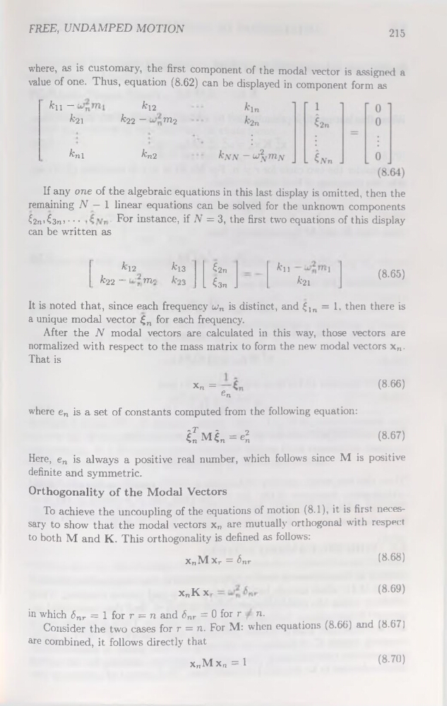
where, as is customary, the first component of the modal vector is assigned a
value of one. Thus, équation (8.62) can be displayed in component form as
fcn -
^21
^nl
^12
fc22 -
W2
^n2
If any one of the algebraic équations in this last display is omitted, then the
remaining TV — 1 linear équations can be solved for the unknown components
€2n>^3n> • • •
For instance, if N = 3, the first two équations of this display
can be written as
*42
fc22 -
m*h3
€2n
À'23
L hn .
fcll
*21
(8.65)
It is noted that, since each frequency ujn is distinct, and £ln = 1. then there is
a unique modal vector £n for each frequency.
After the N modal vectors are calculated in this way, those vectors are
normalized with respect to the mass matrix to form the new modal vectors xn.
That is
x„ =
(8.66)
^n.
where en is a set of constants computed from the following équation:
îlMê„=e2 „
(8.67)
Here, en is always a positive real number, which follows since M is positive
definite and symmetric.
Orthogonality of the Modal Vectors
To achieve the uncoupling of the équations of motion (8.1), it is first necessary to show that the modal vectors xn are mutually orthogonal with respect
to both M and K. This orthogonality is defined as follows:
xnMxr=<5nr
(8.68)
xnK x
(8.69)
in which 6nr = 1 for r = n and 6nr = 0 for r n.
Consider the two cases for r = n. For M: when équations (8.66) and (8.67)
are combined, it follows directly that
x„Mx„ = l
(8-70)
215
where, as is customary, the first component of the modal vector is assigned a
value of one. Thus, équation (8.62) can be displayed in component form as
fcn -
^21
^nl
^12
fc22 -
W2
^n2
If any one of the algebraic équations in this last display is omitted, then the
remaining TV — 1 linear équations can be solved for the unknown components
€2n>^3n> • • •
For instance, if N = 3, the first two équations of this display
can be written as
*42
fc22 -
m*h3
€2n
À'23
L hn .
fcll
*21
(8.65)
It is noted that, since each frequency ujn is distinct, and £ln = 1. then there is
a unique modal vector £n for each frequency.
After the N modal vectors are calculated in this way, those vectors are
normalized with respect to the mass matrix to form the new modal vectors xn.
That is
x„ =
(8.66)
^n.
where en is a set of constants computed from the following équation:
îlMê„=e2 „
(8.67)
Here, en is always a positive real number, which follows since M is positive
definite and symmetric.
Orthogonality of the Modal Vectors
To achieve the uncoupling of the équations of motion (8.1), it is first necessary to show that the modal vectors xn are mutually orthogonal with respect
to both M and K. This orthogonality is defined as follows:
xnMxr=<5nr
(8.68)
xnK x
(8.69)
in which 6nr = 1 for r = n and 6nr = 0 for r n.
Consider the two cases for r = n. For M: when équations (8.66) and (8.67)
are combined, it follows directly that
x„Mx„ = l
(8-70)