

TRANSFER FUNCTIONS FOR WAVE LOADING
95
sin (a + 0) = sin a cos 0 + cos a sin 0
(4.24c)
where a and 0 are real numbers.
The square of the modulas of G(w), needed later for statistical response
studies of structures, is defined by
1G(w)I2 = g(w)-g’(w)
(4.26)
Here G* (w) is the complex conjugate of G(w) and is formed by replacing j by — j
in the transfer function. The calculation of transfer functions is now illustrated
with two example problems.
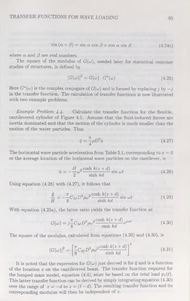
Example Problem 4-4Calculate the transfer function for the flexible,
cantilevered cylinder of Figure 4.1. Assume that the fluid-induced forces are
inertia dominated and that the motion of the cylinder is much smaller than the
motion of the water particles. Thus
K rPq = -pD u
•I
(4-27)
The horizontal wave particle accélération from Table 3.1, corresponding to x = 0
or the average location of the horizontal wave particles on the cantilever, is
H 9 cosh kl z + d) .
u =----- or--------- : -------- sin ait
2
sinh kd
(4-28)
Using équation (4.28) with (4.27), it follows that
H
TT
rP.
2cosh^(2 + ^)
■(-Mu
------, ,----8
sinh kd
sin ait
(4.29)
With équation (4.25a), the latter ratio yields the transfer function as
G(cv) =jlcMD2pJC°Sh k^d)^
(4.30)
8
sinh kd
The square of the modulus, calculated from équations (4.26) and (4.30), is
2
.,2
2cosh^(z + d)
|CM|’ =
Blnh' M -]
(4.31)
It is noted that the expression for G(w) just derived is for q and is a function
of the location z on the cantilevered beam. The transfer function required for
the lumped mass model, équation (4.4), must be based on the total load pi(t).
This latter transfer function can be derived by simply intégrâting équation (4.30)
over the range of z — -d to z = (f - d). The resulting transfer function and its
corresponding modulus will then be independent of z.
95
sin (a + 0) = sin a cos 0 + cos a sin 0
(4.24c)
where a and 0 are real numbers.
The square of the modulas of G(w), needed later for statistical response
studies of structures, is defined by
1G(w)I2 = g(w)-g’(w)
(4.26)
Here G* (w) is the complex conjugate of G(w) and is formed by replacing j by — j
in the transfer function. The calculation of transfer functions is now illustrated
with two example problems.
Example Problem 4-4Calculate the transfer function for the flexible,
cantilevered cylinder of Figure 4.1. Assume that the fluid-induced forces are
inertia dominated and that the motion of the cylinder is much smaller than the
motion of the water particles. Thus
K rPq = -pD u
•I
(4-27)
The horizontal wave particle accélération from Table 3.1, corresponding to x = 0
or the average location of the horizontal wave particles on the cantilever, is
H 9 cosh kl z + d) .
u =----- or--------- : -------- sin ait
2
sinh kd
(4-28)
Using équation (4.28) with (4.27), it follows that
H
TT
rP.
2cosh^(2 + ^)
■(-Mu
------, ,----8
sinh kd
sin ait
(4.29)
With équation (4.25a), the latter ratio yields the transfer function as
G(cv) =jlcMD2pJC°Sh k^d)^
(4.30)
8
sinh kd
The square of the modulus, calculated from équations (4.26) and (4.30), is
2
.,2
2cosh^(z + d)
|CM|’ =
Blnh' M -]
(4.31)
It is noted that the expression for G(w) just derived is for q and is a function
of the location z on the cantilevered beam. The transfer function required for
the lumped mass model, équation (4.4), must be based on the total load pi(t).
This latter transfer function can be derived by simply intégrâting équation (4.30)
over the range of z — -d to z = (f - d). The resulting transfer function and its
corresponding modulus will then be independent of z.