

in a turning of the height contours of the lake surface. Howeyer, the
turning of the contours lagged behind the wind so that for a time the
wind blew parallel to the water level contours instead of perpendicular
to them. Contour lines of the lake surface from 1800 hours on 26 August
to 0600 hours on 27 August 1949 are shown in.Figure 3-57. The map contours for 2300 hours on 26 August show the wind blowing parallel to the
highest contours at two locations. (Haurwitz, 1951), (Saville, 1952),?(Sibul, 1955), (Tickner, 1957), and (U.S. Army, Corps of Engineers, 1955).)
Recorded examples of wind setup on the Great Lakes are available from
the U.S. Lake Survey, National Océan Survey, and NOAA. These observations
hâve been used for the development of theoretical methods for forecasting
water levels during approaching storms and for the planning and design of
engineering works. As a resuit of the need to predict unusually high
stages on the Great Lakes, numerous theoretical investigations hâve been
made of wind setup for that area. (Harris, 1953), (Harris and Angelo,
1962), (Platzman and Rao, 1963), (Jelesnianski, 1958), (Irish and
Platzman, 1962), and (Platzman, 1958, 1963, 1965, and 1967).)
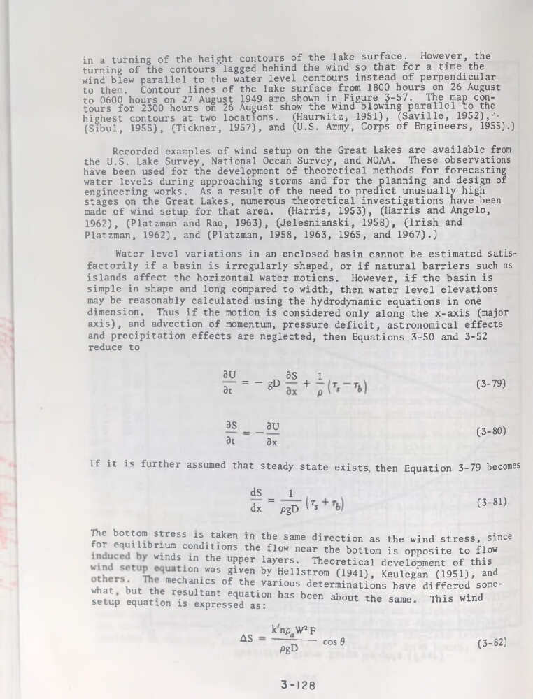
Water level variations in an enclosed basin cannot be estimated satisfactorily if a basin is irregularly shaped, or if natural barriers such as
islands affect the horizontal water motions. However, if the basin is
simple in shape and long compared to width, then water level élévations
may be reasonably calculated using the hydrodynamic équations in one
dimension. Thus if the motion is considered only along the x-axis (major
axis), and advection of momentum, pressure déficit, astronomical effects
and précipitation effects are neglected, then Equations 3-50 and 3-52
reduce to
dU _
9S
1
3t _ "gD
+
(3-79)
ds___ au
dt
dx
(3-80)
If it is further assumed that steady State exists, then Equation 3-79 becomes
dS = 1
dx
pgD 'T*
(3-81)
pie bottom stress is taken in the same direction as the wind stress, since
for equilibnum conditions the flow near the bottom is opposite to flow
Wlnd*.ln the uPPer layers. Theoretical development of this
h°n WaS !1Ven by Hellstrom (1941), Keulegan (1951), and
what hi
mecha"lcs of the various déterminations hâve differed somewhat but the résultant équation has been about the same
This wind
setup équation is expressed as:
knp W2F
△S
~----- cos 6
PgD
(3-82)
3-128
turning of the contours lagged behind the wind so that for a time the
wind blew parallel to the water level contours instead of perpendicular
to them. Contour lines of the lake surface from 1800 hours on 26 August
to 0600 hours on 27 August 1949 are shown in.Figure 3-57. The map contours for 2300 hours on 26 August show the wind blowing parallel to the
highest contours at two locations. (Haurwitz, 1951), (Saville, 1952),?(Sibul, 1955), (Tickner, 1957), and (U.S. Army, Corps of Engineers, 1955).)
Recorded examples of wind setup on the Great Lakes are available from
the U.S. Lake Survey, National Océan Survey, and NOAA. These observations
hâve been used for the development of theoretical methods for forecasting
water levels during approaching storms and for the planning and design of
engineering works. As a resuit of the need to predict unusually high
stages on the Great Lakes, numerous theoretical investigations hâve been
made of wind setup for that area. (Harris, 1953), (Harris and Angelo,
1962), (Platzman and Rao, 1963), (Jelesnianski, 1958), (Irish and
Platzman, 1962), and (Platzman, 1958, 1963, 1965, and 1967).)
Water level variations in an enclosed basin cannot be estimated satisfactorily if a basin is irregularly shaped, or if natural barriers such as
islands affect the horizontal water motions. However, if the basin is
simple in shape and long compared to width, then water level élévations
may be reasonably calculated using the hydrodynamic équations in one
dimension. Thus if the motion is considered only along the x-axis (major
axis), and advection of momentum, pressure déficit, astronomical effects
and précipitation effects are neglected, then Equations 3-50 and 3-52
reduce to
dU _
9S
1
3t _ "gD
+
(3-79)
ds___ au
dt
dx
(3-80)
If it is further assumed that steady State exists, then Equation 3-79 becomes
dS = 1
dx
pgD 'T*
(3-81)
pie bottom stress is taken in the same direction as the wind stress, since
for equilibnum conditions the flow near the bottom is opposite to flow
Wlnd*.ln the uPPer layers. Theoretical development of this
h°n WaS !1Ven by Hellstrom (1941), Keulegan (1951), and
what hi
mecha"lcs of the various déterminations hâve differed somewhat but the résultant équation has been about the same
This wind
setup équation is expressed as:
knp W2F
△S
~----- cos 6
PgD
(3-82)
3-128