

of metres and below dominate the surface boundary layer, and ultimately determine the overall
strength of the thermohaline circulation at long
time scales.
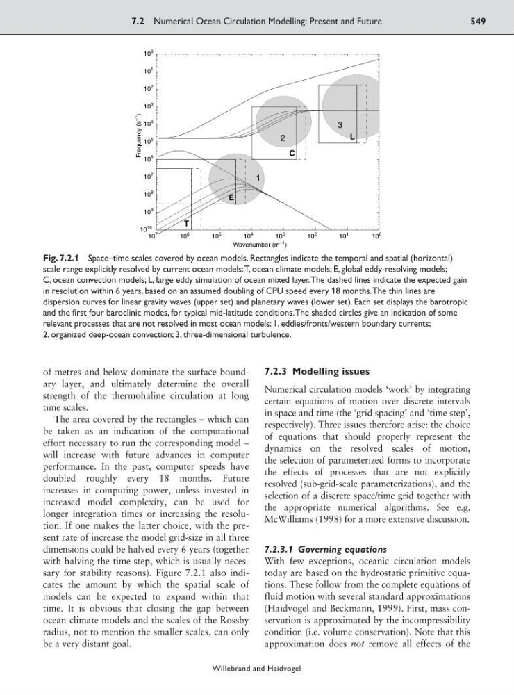
The area covered by the rectangles – which can
be taken as an indication of the computational
effort necessary to run the corresponding model –
will increase with future advances in computer
performance. In the past, computer speeds have
doubled roughly every 18 months. Future
increases in computing power, unless invested in
increased model complexity, can be used for
longer integration times or increasing the resolution. If one makes the latter choice, with the present rate of increase the model grid-size in all three
dimensions could be halved every 6 years (together
with halving the time step, which is usually necessary for stability reasons). Figure 7.2.1 also indicates the amount by which the spatial scale of
models can be expected to expand within that
time. It is obvious that closing the gap between
ocean climate models and the scales of the Rossby
radius, not to mention the smaller scales, can only
be a very distant goal.
7.2.3 Modelling issues
Numerical circulation models ‘work’ by integrating
certain equations of motion over discrete intervals
in space and time (the ‘grid spacing’ and ‘time step’,
respectively). Three issues therefore arise: the choice
of equations that should properly represent the
dynamics on the resolved scales of motion,
the selection of parameterized forms to incorporate
the effects of processes that are not explicitly
resolved (sub-grid-scale parameterizations), and the
selection of a discrete space/time grid together with
the appropriate numerical algorithms. See e.g.
McWilliams (1998) for a more extensive discussion.
7.2.3.1 Governing equations
With few exceptions, oceanic circulation models
today are based on the hydrostatic primitive equations. These follow from the complete equations of
fluid motion with several standard approximations
(Haidvogel and Beckmann, 1999). First, mass conservation is approximated by the incompressibility
condition (i.e. volume conservation). Note that this
approximation does not remove all effects of the
7.2 Numerical Ocean Circulation Modelling: Present and Future
549
Willebrand and Haidvogel
10
7
10
6
10
5
10
4
10
3
10
2
10
1
10
0
10
10
10
9
10
8
10
7
10
6
10
5
10
4
10
3
10
2
10
1
10
0
Wavenumber (m
–1 )
Frequency (s
–1
)
1
2
3
T
E
C
L
Fig. 7.2.1 Space–time scales covered by ocean models. Rectangles indicate the temporal and spatial (horizontal)
scale range explicitly resolved by current ocean models:T, ocean climate models; E, global eddy-resolving models;
C, ocean convection models; L, large eddy simulation of ocean mixed layer.The dashed lines indicate the expected gain
in resolution within 6 years, based on an assumed doubling of CPU speed every 18 months.The thin lines are
dispersion curves for linear gravity waves (upper set) and planetary waves (lower set). Each set displays the barotropic
and the first four baroclinic modes, for typical mid-latitude conditions.The shaded circles give an indication of some
relevant processes that are not resolved in most ocean models: 1, eddies/fronts/western boundary currents;
2, organized deep-ocean convection; 3, three-dimensional turbulence.
strength of the thermohaline circulation at long
time scales.
The area covered by the rectangles – which can
be taken as an indication of the computational
effort necessary to run the corresponding model –
will increase with future advances in computer
performance. In the past, computer speeds have
doubled roughly every 18 months. Future
increases in computing power, unless invested in
increased model complexity, can be used for
longer integration times or increasing the resolution. If one makes the latter choice, with the present rate of increase the model grid-size in all three
dimensions could be halved every 6 years (together
with halving the time step, which is usually necessary for stability reasons). Figure 7.2.1 also indicates the amount by which the spatial scale of
models can be expected to expand within that
time. It is obvious that closing the gap between
ocean climate models and the scales of the Rossby
radius, not to mention the smaller scales, can only
be a very distant goal.
7.2.3 Modelling issues
Numerical circulation models ‘work’ by integrating
certain equations of motion over discrete intervals
in space and time (the ‘grid spacing’ and ‘time step’,
respectively). Three issues therefore arise: the choice
of equations that should properly represent the
dynamics on the resolved scales of motion,
the selection of parameterized forms to incorporate
the effects of processes that are not explicitly
resolved (sub-grid-scale parameterizations), and the
selection of a discrete space/time grid together with
the appropriate numerical algorithms. See e.g.
McWilliams (1998) for a more extensive discussion.
7.2.3.1 Governing equations
With few exceptions, oceanic circulation models
today are based on the hydrostatic primitive equations. These follow from the complete equations of
fluid motion with several standard approximations
(Haidvogel and Beckmann, 1999). First, mass conservation is approximated by the incompressibility
condition (i.e. volume conservation). Note that this
approximation does not remove all effects of the
7.2 Numerical Ocean Circulation Modelling: Present and Future
549
Willebrand and Haidvogel
10
7
10
6
10
5
10
4
10
3
10
2
10
1
10
0
10
10
10
9
10
8
10
7
10
6
10
5
10
4
10
3
10
2
10
1
10
0
Wavenumber (m
–1 )
Frequency (s
–1
)
1
2
3
T
E
C
L
Fig. 7.2.1 Space–time scales covered by ocean models. Rectangles indicate the temporal and spatial (horizontal)
scale range explicitly resolved by current ocean models:T, ocean climate models; E, global eddy-resolving models;
C, ocean convection models; L, large eddy simulation of ocean mixed layer.The dashed lines indicate the expected gain
in resolution within 6 years, based on an assumed doubling of CPU speed every 18 months.The thin lines are
dispersion curves for linear gravity waves (upper set) and planetary waves (lower set). Each set displays the barotropic
and the first four baroclinic modes, for typical mid-latitude conditions.The shaded circles give an indication of some
relevant processes that are not resolved in most ocean models: 1, eddies/fronts/western boundary currents;
2, organized deep-ocean convection; 3, three-dimensional turbulence.