

(or, more accurately, temporal differences in the
spatial pattern of residuals) are therefore interpreted as reflecting additional ‘non-natural’
TCO 2 variability, primarily that resulting from
a temporal increase in the Excess CO 2 concentration of seawater.
¥ In the case of comparisons with historical data
sets, systematic calibration errors of the earlier
data are to be expected. Such offsets appear as
systematic non-zero values for residuals in deep
waters where the increase of Excess CO 2 over
time should usually be small. Such deep-water
residuals from GEOSECS-WOCE data comparisons, in depth ranges where transient tracers
such as the CFCs and CCl 4 are absent, were
interpreted as a TCO 2 calibration errors with
the GEOSECS data (Wallace, 1995; Sabine
et al., 1999). The GEOSECS data were accordingly corrected throughout the water column
for this deep-water offset.
This approach allows all available data to
be compared and relaxes certain assumptions of
the preformed techniques: notably no particular
value for the stoichiometric relationship between
oxygen utilization and TCO 2 increase is assumed –
rather a value is estimated empirically from the
data (as a partial regression coefficient). Wallace
(1995) examined this residual variability in the
western basin of the South Atlantic subtropical
gyre based on data collected in 1973–74 during
GEOSECS, during 1988–89 during SAVE, and
along WOCE A8 (11°S), A9 (19°S) and A10 (30°S)
during 1991–93. The vertical profiles of the TCO 2
residuals resulting from this comparison closely
matched what might be expected for a profile of
Excess CO 2 increase over 20 years based on the
distribution of CFC-11. Sabine et al. (1999) subsequently applied this approach to the Indian Ocean
survey TCO 2 data in comparison with GEOSECS.
The distribution of the temporal build-up of
Excess CO 2 calculated in this empirical way
closely matched the distribution estimated using
the inventory approach (see Fig. 6.3.10b).
A data selection and correction approach
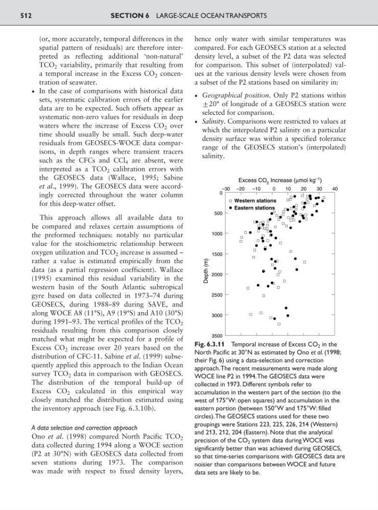
Ono et al. (1998) compared North Pacific TCO 2
data collected during 1994 along a WOCE section
(P2 at 30°N) with GEOSECS data collected from
seven stations during 1973. The comparison
was made with respect to fixed density layers,
hence only water with similar temperatures was
compared. For each GEOSECS station at a selected
density level, a subset of the P2 data was selected
for comparison. This subset of (interpolated) values at the various density levels were chosen from
a subset of the P2 stations based on similarity in:
¥ Geographical position. Only P2 stations within
<20° of longitude of a GEOSECS station were
selected for comparison.
¥ Salinity. Comparisons were restricted to values at
which the interpolated P2 salinity on a particular
density surface was within a specified tolerance
range of the GEOSECS station’s (interpolated)
salinity.
SECTION 6 LARGE-SCALE OCEAN TRANSPORTS
512
Excess CO 2 Increase (μmol kg
–1 )
–30 –20
–10
10
20
30
40
Depth (m)
0
500
1000
1500
2000
2500
3000
3500
Eastern stations
Western stations
0
Fig. 6.3.11 Temporal increase of Excess CO 2 in the
North Pacific at 30°N as estimated by Ono et al. (1998;
their Fig. 6) using a data-selection and correction
approach.The recent measurements were made along
WOCE line P2 in 1994.The GEOSECS data were
collected in 1973. Different symbols refer to
accumulation in the western part of the section (to the
west of 175°W: open squares) and accumulation in the
eastern portion (between 150°W and 175°W: filled
circles).The GEOSECS stations used for these two
groupings were Stations 223, 225, 226, 214 (Western)
and 213, 212, 204 (Eastern). Note that the analytical
precision of the CO 2 system data during WOCE was
significantly better than was achieved during GEOSECS,
so that time-series comparisons with GEOSECS data are
noisier than comparisons between WOCE and future
data sets are likely to be.
spatial pattern of residuals) are therefore interpreted as reflecting additional ‘non-natural’
TCO 2 variability, primarily that resulting from
a temporal increase in the Excess CO 2 concentration of seawater.
¥ In the case of comparisons with historical data
sets, systematic calibration errors of the earlier
data are to be expected. Such offsets appear as
systematic non-zero values for residuals in deep
waters where the increase of Excess CO 2 over
time should usually be small. Such deep-water
residuals from GEOSECS-WOCE data comparisons, in depth ranges where transient tracers
such as the CFCs and CCl 4 are absent, were
interpreted as a TCO 2 calibration errors with
the GEOSECS data (Wallace, 1995; Sabine
et al., 1999). The GEOSECS data were accordingly corrected throughout the water column
for this deep-water offset.
This approach allows all available data to
be compared and relaxes certain assumptions of
the preformed techniques: notably no particular
value for the stoichiometric relationship between
oxygen utilization and TCO 2 increase is assumed –
rather a value is estimated empirically from the
data (as a partial regression coefficient). Wallace
(1995) examined this residual variability in the
western basin of the South Atlantic subtropical
gyre based on data collected in 1973–74 during
GEOSECS, during 1988–89 during SAVE, and
along WOCE A8 (11°S), A9 (19°S) and A10 (30°S)
during 1991–93. The vertical profiles of the TCO 2
residuals resulting from this comparison closely
matched what might be expected for a profile of
Excess CO 2 increase over 20 years based on the
distribution of CFC-11. Sabine et al. (1999) subsequently applied this approach to the Indian Ocean
survey TCO 2 data in comparison with GEOSECS.
The distribution of the temporal build-up of
Excess CO 2 calculated in this empirical way
closely matched the distribution estimated using
the inventory approach (see Fig. 6.3.10b).
A data selection and correction approach
Ono et al. (1998) compared North Pacific TCO 2
data collected during 1994 along a WOCE section
(P2 at 30°N) with GEOSECS data collected from
seven stations during 1973. The comparison
was made with respect to fixed density layers,
hence only water with similar temperatures was
compared. For each GEOSECS station at a selected
density level, a subset of the P2 data was selected
for comparison. This subset of (interpolated) values at the various density levels were chosen from
a subset of the P2 stations based on similarity in:
¥ Geographical position. Only P2 stations within
<20° of longitude of a GEOSECS station were
selected for comparison.
¥ Salinity. Comparisons were restricted to values at
which the interpolated P2 salinity on a particular
density surface was within a specified tolerance
range of the GEOSECS station’s (interpolated)
salinity.
SECTION 6 LARGE-SCALE OCEAN TRANSPORTS
512
Excess CO 2 Increase (μmol kg
–1 )
–30 –20
–10
10
20
30
40
Depth (m)
0
500
1000
1500
2000
2500
3000
3500
Eastern stations
Western stations
0
Fig. 6.3.11 Temporal increase of Excess CO 2 in the
North Pacific at 30°N as estimated by Ono et al. (1998;
their Fig. 6) using a data-selection and correction
approach.The recent measurements were made along
WOCE line P2 in 1994.The GEOSECS data were
collected in 1973. Different symbols refer to
accumulation in the western part of the section (to the
west of 175°W: open squares) and accumulation in the
eastern portion (between 150°W and 175°W: filled
circles).The GEOSECS stations used for these two
groupings were Stations 223, 225, 226, 214 (Western)
and 213, 212, 204 (Eastern). Note that the analytical
precision of the CO 2 system data during WOCE was
significantly better than was achieved during GEOSECS,
so that time-series comparisons with GEOSECS data are
noisier than comparisons between WOCE and future
data sets are likely to be.