

unconfirmed until now (Niiler and Barth, 2001).
There was no significant mean current system
within 1° of the equator, contrary to every existing
mean ocean current chart now in use. The South
Equatorial Current vanished on the equator and
had a maximum on either side of the equator. The
remarkable steadiness of the Pacific North Equatorial Current, west of the dateline, and the South
Equatorial Current in the eastern Pacific, were neither anticipated nor demon- strated by the ship
drift charts of those regions (Wyrtki et al., 1976).
As an example of how the picture of circulation
on Fig. 4.1.5a changes with changing spatial resolution, a chart using 1°1° binned data was made
for the western North Pacific (Fig. 4.1.5b, see Plate
4.1.5b, p. 300) and western North Atlantic (Fig.
4.1.5c, see Plate 4.1.5c, p. 300). In both oceans, a
countercurrent can be discerned at 21–23° latitude.
These subtropical countercurrents were predicted
to exist from the high-resolution hydrographic
data, for example as shown by White and Walker
(1985), but had not been evident in ship-drift
charts. Along the western North Pacific boundary,
a significant flow was found from the North Equatorial Current to the South China Sea between
Taiwan and Mindanao. This latter pathway of
water exchange between the Pacific and the Indian
Oceans has not been explored as carefully as the
pathways through the Indonesian archipelago. The
steadiness of the North Equatorial Current is further in evidence in the spatial ‘smoothness’ of the
vectors at this high resolution. There were a number of features of the continuity and discontinuity
of the surface flow between the major current systems that require an examination of the detailed
tracks of the drifters, a task that requires even
higher resolution in space and time than has been
done here. The data similar to those displayed on
Figs 4.1.5a and 4.1.5b,c will continue to be examined with more scrutiny for discoveries of circulation features than can be done in this treatise. It
suffices here to state that the calibrated instrumental observations of ocean circulation on a global
basis will continue not only to discover circulation
patterns not seen before, but also to map these and
those familiar to mariners with great accuracy.
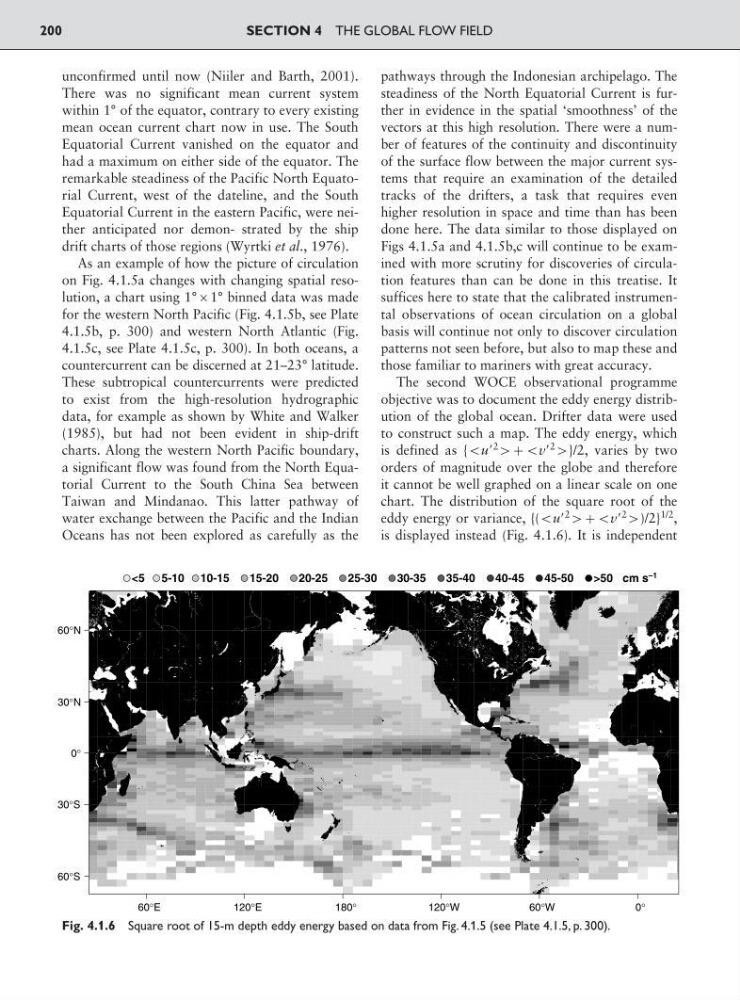
The second WOCE observational programme
objective was to document the eddy energy distribution of the global ocean. Drifter data were used
to construct such a map. The eddy energy, which
is defined as {:uЈ
2
9;:vЈ
2
9}/2, varies by two
orders of magnitude over the globe and therefore
it cannot be well graphed on a linear scale on one
chart. The distribution of the square root of the
eddy energy or variance, {(:uЈ
2
9;:vЈ
2
9)/2}
1/2 ,
is displayed instead (Fig. 4.1.6). It is independent
SECTION 4 THE GLOBAL FLOW FIELD
200
60°E
120°E
180°
120°W
60°W
0°
60°S
30°S
0°
30°N
60°N
<5 5-10 10-15
15-20
20-25
25-30
30-35
35-40
40-45
45-50
>50 cm s
–1
Fig. 4.1.6 Square root of 15-m depth eddy energy based on data from Fig. 4.1.5 (see Plate 4.1.5, p. 300).
There was no significant mean current system
within 1° of the equator, contrary to every existing
mean ocean current chart now in use. The South
Equatorial Current vanished on the equator and
had a maximum on either side of the equator. The
remarkable steadiness of the Pacific North Equatorial Current, west of the dateline, and the South
Equatorial Current in the eastern Pacific, were neither anticipated nor demon- strated by the ship
drift charts of those regions (Wyrtki et al., 1976).
As an example of how the picture of circulation
on Fig. 4.1.5a changes with changing spatial resolution, a chart using 1°1° binned data was made
for the western North Pacific (Fig. 4.1.5b, see Plate
4.1.5b, p. 300) and western North Atlantic (Fig.
4.1.5c, see Plate 4.1.5c, p. 300). In both oceans, a
countercurrent can be discerned at 21–23° latitude.
These subtropical countercurrents were predicted
to exist from the high-resolution hydrographic
data, for example as shown by White and Walker
(1985), but had not been evident in ship-drift
charts. Along the western North Pacific boundary,
a significant flow was found from the North Equatorial Current to the South China Sea between
Taiwan and Mindanao. This latter pathway of
water exchange between the Pacific and the Indian
Oceans has not been explored as carefully as the
pathways through the Indonesian archipelago. The
steadiness of the North Equatorial Current is further in evidence in the spatial ‘smoothness’ of the
vectors at this high resolution. There were a number of features of the continuity and discontinuity
of the surface flow between the major current systems that require an examination of the detailed
tracks of the drifters, a task that requires even
higher resolution in space and time than has been
done here. The data similar to those displayed on
Figs 4.1.5a and 4.1.5b,c will continue to be examined with more scrutiny for discoveries of circulation features than can be done in this treatise. It
suffices here to state that the calibrated instrumental observations of ocean circulation on a global
basis will continue not only to discover circulation
patterns not seen before, but also to map these and
those familiar to mariners with great accuracy.
The second WOCE observational programme
objective was to document the eddy energy distribution of the global ocean. Drifter data were used
to construct such a map. The eddy energy, which
is defined as {:uЈ
2
9;:vЈ
2
9}/2, varies by two
orders of magnitude over the globe and therefore
it cannot be well graphed on a linear scale on one
chart. The distribution of the square root of the
eddy energy or variance, {(:uЈ
2
9;:vЈ
2
9)/2}
1/2 ,
is displayed instead (Fig. 4.1.6). It is independent
SECTION 4 THE GLOBAL FLOW FIELD
200
60°E
120°E
180°
120°W
60°W
0°
60°S
30°S
0°
30°N
60°N
<5 5-10 10-15
15-20
20-25
25-30
30-35
35-40
40-45
45-50
>50 cm s
–1
Fig. 4.1.6 Square root of 15-m depth eddy energy based on data from Fig. 4.1.5 (see Plate 4.1.5, p. 300).