

The empirical form of the original scatterometer
algorithm leads to an asymptotic decrease in the
sensitivity in scatterometer-derived winds for
higher wind speeds (Cavanié and Lecomte, 1987).
Insufficient measurements in the past prevented
significant improvement of wind retrieval for wind
speeds over 25 m s
91
. Quilfen et al. (1998) illustrated with the C-band AMI data, at 25 km resolution, obtained for a special 20-orbit data set, that
the backscatter cross-section continues to show
sensitivity beyond 20 m s
91 winds in tropical
cyclones. Similarly, Yueh et al. (2000) have shown
that a Ku-band scatterometer is sensitive to both
wind speed and direction under hurricane conditions, with wind speeds up to 35 m s
91 . Improvement of the wind-retrieval algorithm under the
strong wind conditions of tropical cyclones is
being vigorously pursued (e.g. Jones et al., 1999b;
Liu et al., 2000).
The equivalent neutral winds produced by
space-borne scatterometers (Liu and Tang, 1996)
are uniquely related to the surface stress by equation (3.4.1). Another valid algorithm approach
relates the backscatter observation directly to measurements of surface stress instead of to the equivalent neutral wind; the feasibility was demonstrated
by Liu and Large (1981), Weissman and Graber
(1999), and others.
The minimum requirements for the US scatterometer are wind speed accuracy of either 10%
or 2 m s
91
, depending on which is larger, and
directional accuracy of 20° in the speed range of
3–10 m s
91
, under all weather conditions except
heavy rain. Freilich and Dunbar (1999) clearly
SECTION 3 NEW WAYS OF OBSERVING THE OCEAN
176
0
5
10
15
20 0
5
10
15
20 0
5
10
15
20
0
5
10
15
20
Bias= 0.02
RMS= 1.22
Corr= 0.91
bs= 0.95
Satellite (m s
–1
)
Bias= 0.57
RMS= 1.49
Corr= 0.81
bs= 0.86
Daily Wind Speed
Bias= 0.56
RMS= 1.76
Corr= 0.88
bs= 0.95
-15 -10
-5
0
5
10 15 -15 -10
-5
0
5
10 15 -15 -10
-5
0
5
10 15
-15 -10
-5
0
5
10 15 -15 -10
-5
0
5
10 15 -15 -10
-5
0
5
10 15
-15
-10
-5
0
5
10
15
Bias= 0.03
RMS= 1.99
Corr= 0.95
bs= 1.15
Satellite (m s
–1
)
-15
-10
-5
0
5
10
15
Satellite (m s
–1
)
Bias= 0.28
RMS= 1.62
Corr= 0.93
bs= 1.06
Daily Zonal Component
Bias= 0.11
RMS= 2.50
Corr= 0.94
bs= 1.24
Bias= 0.21
RMS= 2.08
Corr= 0.90
bs= 1.10
NDBC (m s
–1 )
Bias= 0.42
RMS= 1.56
Corr= 0.85
bs= 1.08
TAO (m s –1 )
Daily Meridional Component
Bias= 0.26
RMS= 2.35
Corr= 0.85
bs= 1.18
ODAS (m s
–1 )
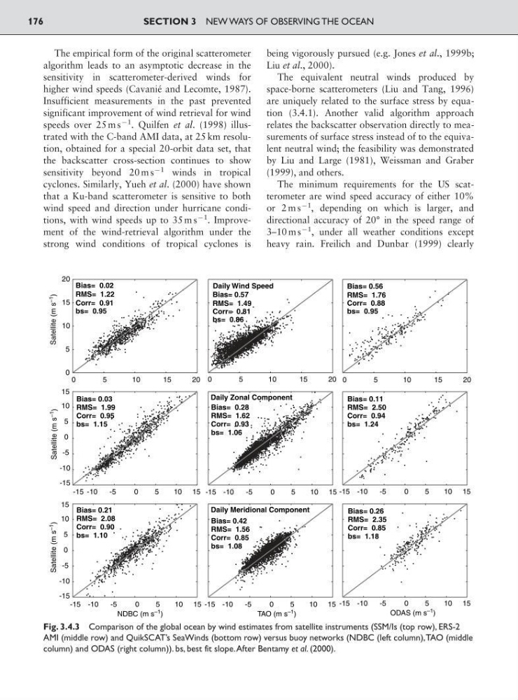
Fig. 3.4.3 Comparison of the global ocean by wind estimates from satellite instruments (SSM/Is (top row), ERS-2
AMI (middle row) and QuikSCAT’s SeaWinds (bottom row) versus buoy networks (NDBC (left column),TAO (middle
column) and ODAS (right column)). bs, best fit slope.After Bentamy et al. (2000).
algorithm leads to an asymptotic decrease in the
sensitivity in scatterometer-derived winds for
higher wind speeds (Cavanié and Lecomte, 1987).
Insufficient measurements in the past prevented
significant improvement of wind retrieval for wind
speeds over 25 m s
91
. Quilfen et al. (1998) illustrated with the C-band AMI data, at 25 km resolution, obtained for a special 20-orbit data set, that
the backscatter cross-section continues to show
sensitivity beyond 20 m s
91 winds in tropical
cyclones. Similarly, Yueh et al. (2000) have shown
that a Ku-band scatterometer is sensitive to both
wind speed and direction under hurricane conditions, with wind speeds up to 35 m s
91 . Improvement of the wind-retrieval algorithm under the
strong wind conditions of tropical cyclones is
being vigorously pursued (e.g. Jones et al., 1999b;
Liu et al., 2000).
The equivalent neutral winds produced by
space-borne scatterometers (Liu and Tang, 1996)
are uniquely related to the surface stress by equation (3.4.1). Another valid algorithm approach
relates the backscatter observation directly to measurements of surface stress instead of to the equivalent neutral wind; the feasibility was demonstrated
by Liu and Large (1981), Weissman and Graber
(1999), and others.
The minimum requirements for the US scatterometer are wind speed accuracy of either 10%
or 2 m s
91
, depending on which is larger, and
directional accuracy of 20° in the speed range of
3–10 m s
91
, under all weather conditions except
heavy rain. Freilich and Dunbar (1999) clearly
SECTION 3 NEW WAYS OF OBSERVING THE OCEAN
176
0
5
10
15
20 0
5
10
15
20 0
5
10
15
20
0
5
10
15
20
Bias= 0.02
RMS= 1.22
Corr= 0.91
bs= 0.95
Satellite (m s
–1
)
Bias= 0.57
RMS= 1.49
Corr= 0.81
bs= 0.86
Daily Wind Speed
Bias= 0.56
RMS= 1.76
Corr= 0.88
bs= 0.95
-15 -10
-5
0
5
10 15 -15 -10
-5
0
5
10 15 -15 -10
-5
0
5
10 15
-15 -10
-5
0
5
10 15 -15 -10
-5
0
5
10 15 -15 -10
-5
0
5
10 15
-15
-10
-5
0
5
10
15
Bias= 0.03
RMS= 1.99
Corr= 0.95
bs= 1.15
Satellite (m s
–1
)
-15
-10
-5
0
5
10
15
Satellite (m s
–1
)
Bias= 0.28
RMS= 1.62
Corr= 0.93
bs= 1.06
Daily Zonal Component
Bias= 0.11
RMS= 2.50
Corr= 0.94
bs= 1.24
Bias= 0.21
RMS= 2.08
Corr= 0.90
bs= 1.10
NDBC (m s
–1 )
Bias= 0.42
RMS= 1.56
Corr= 0.85
bs= 1.08
TAO (m s –1 )
Daily Meridional Component
Bias= 0.26
RMS= 2.35
Corr= 0.85
bs= 1.18
ODAS (m s
–1 )
Fig. 3.4.3 Comparison of the global ocean by wind estimates from satellite instruments (SSM/Is (top row), ERS-2
AMI (middle row) and QuikSCAT’s SeaWinds (bottom row) versus buoy networks (NDBC (left column),TAO (middle
column) and ODAS (right column)). bs, best fit slope.After Bentamy et al. (2000).