

cold event of 11 000 years BP (Broecker, 1997).
Such behaviour has been shown in the GFDL
GCM (Manabe and Stouffer, 1988, 1997) as well
as in the intermediate complexity CLIMBER
model (Rahmstorf and Ganopolski, 1999 – see
Section 2.3.2.1). Much of the modelling uncertainty arises because the THC response is controlled by the sum of a number of positive and
negative feedbacks. These feedbacks have been
extensively studied in simple models but have not
as yet been systematically quantified in GCMs (see
Rahmstorf et al., 1996, for a review).
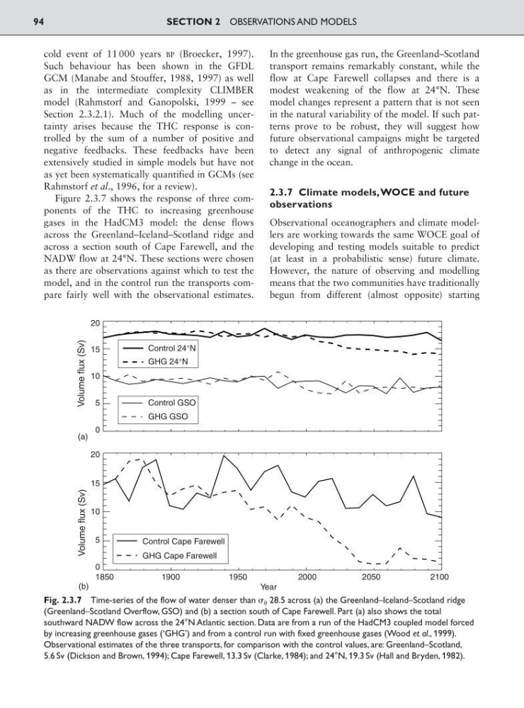
Figure 2.3.7 shows the response of three components of the THC to increasing greenhouse
gases in the HadCM3 model: the dense flows
across the Greenland–Iceland–Scotland ridge and
across a section south of Cape Farewell, and the
NADW flow at 24°N. These sections were chosen
as there are observations against which to test the
model, and in the control run the transports compare fairly well with the observational estimates.
In the greenhouse gas run, the Greenland–Scotland
transport remains remarkably constant, while the
flow at Cape Farewell collapses and there is a
modest weakening of the flow at 24°N. These
model changes represent a pattern that is not seen
in the natural variability of the model. If such patterns prove to be robust, they will suggest how
future observational campaigns might be targeted
to detect any signal of anthropogenic climate
change in the ocean.
2.3.7 Climate models,WOCE and future
observations
Observational oceanographers and climate modellers are working towards the same WOCE goal of
developing and testing models suitable to predict
(at least in a probabilistic sense) future climate.
However, the nature of observing and modelling
means that the two communities have traditionally
begun from different (almost opposite) starting
SECTION 2 OBSERVATIONS AND MODELS
94
Control 24°N
Control GSO
Control Cape Farewell
GHG 24°N
GHG GSO
GHG Cape Farewell
20
15
10
5
0
(a)
(b)
Volume flux (Sv)
20
15
10
5
0
Volume flux (Sv)
1850
1900
1950
2000
2050
2100
Year
Fig. 2.3.7 Time-series of the flow of water denser than 28.5 across (a) the Greenland–Iceland–Scotland ridge
(Greenland–Scotland Overflow, GSO) and (b) a section south of Cape Farewell. Part (a) also shows the total
southward NADW flow across the 24°N Atlantic section. Data are from a run of the HadCM3 coupled model forced
by increasing greenhouse gases (‘GHG’) and from a control run with fixed greenhouse gases (Wood et al., 1999).
Observational estimates of the three transports, for comparison with the control values, are: Greenland–Scotland,
5.6 Sv (Dickson and Brown, 1994); Cape Farewell, 13.3 Sv (Clarke, 1984); and 24°N, 19.3 Sv (Hall and Bryden, 1982).
Such behaviour has been shown in the GFDL
GCM (Manabe and Stouffer, 1988, 1997) as well
as in the intermediate complexity CLIMBER
model (Rahmstorf and Ganopolski, 1999 – see
Section 2.3.2.1). Much of the modelling uncertainty arises because the THC response is controlled by the sum of a number of positive and
negative feedbacks. These feedbacks have been
extensively studied in simple models but have not
as yet been systematically quantified in GCMs (see
Rahmstorf et al., 1996, for a review).
Figure 2.3.7 shows the response of three components of the THC to increasing greenhouse
gases in the HadCM3 model: the dense flows
across the Greenland–Iceland–Scotland ridge and
across a section south of Cape Farewell, and the
NADW flow at 24°N. These sections were chosen
as there are observations against which to test the
model, and in the control run the transports compare fairly well with the observational estimates.
In the greenhouse gas run, the Greenland–Scotland
transport remains remarkably constant, while the
flow at Cape Farewell collapses and there is a
modest weakening of the flow at 24°N. These
model changes represent a pattern that is not seen
in the natural variability of the model. If such patterns prove to be robust, they will suggest how
future observational campaigns might be targeted
to detect any signal of anthropogenic climate
change in the ocean.
2.3.7 Climate models,WOCE and future
observations
Observational oceanographers and climate modellers are working towards the same WOCE goal of
developing and testing models suitable to predict
(at least in a probabilistic sense) future climate.
However, the nature of observing and modelling
means that the two communities have traditionally
begun from different (almost opposite) starting
SECTION 2 OBSERVATIONS AND MODELS
94
Control 24°N
Control GSO
Control Cape Farewell
GHG 24°N
GHG GSO
GHG Cape Farewell
20
15
10
5
0
(a)
(b)
Volume flux (Sv)
20
15
10
5
0
Volume flux (Sv)
1850
1900
1950
2000
2050
2100
Year
Fig. 2.3.7 Time-series of the flow of water denser than 28.5 across (a) the Greenland–Iceland–Scotland ridge
(Greenland–Scotland Overflow, GSO) and (b) a section south of Cape Farewell. Part (a) also shows the total
southward NADW flow across the 24°N Atlantic section. Data are from a run of the HadCM3 coupled model forced
by increasing greenhouse gases (‘GHG’) and from a control run with fixed greenhouse gases (Wood et al., 1999).
Observational estimates of the three transports, for comparison with the control values, are: Greenland–Scotland,
5.6 Sv (Dickson and Brown, 1994); Cape Farewell, 13.3 Sv (Clarke, 1984); and 24°N, 19.3 Sv (Hall and Bryden, 1982).