

ANALYSIS O F PROCESSES IN CONTROL OF INSECTS
21
geometric increase at two different rates, i.e. there is no densitydependent effect. Plotting log N , versus log N,+l for these, after
reading off the values from the graph of C and I), gives the two lines
C’ and D’ in Fig. 9 ~ ,
both with a slope of 1. Curves E and P represent
increase which decelerates, on the geometric or logarithmic scale, as
density increases; such a pattern, if it is established as not being due
to some progressive change in weather, etc., would be interpreted as a
density-dependent phenomenon. The corresponding lines E’ and F’
each have a slope less than unity, and the more strongly densitydependent F’ has a lower slope than E‘. Curve G represents the effect
of an inverse relationship ; the rate of geometric increase rises as density
rises. The slope of the corresponding line G is greater than 1, approximately 2.0. It may seem unrealistic to introduce this example, since a
population of this sort would be inherently unstable. However, such
relationships do occur, often as a temporary phase.
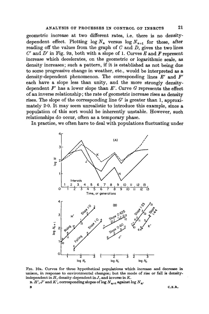
In practice, we often have to deal with populations fluctuating under
1 1 , 2 , 3., 4 , 5 , 6 , 7 , 8 , 9 , l o , I I , 1 2 , 1 3 ,
0
1
2 3 4 5 6 7 8 9 1 0 I I 12 1 3
Time, or generotions
0
2
L -
1
2
3 1
2
3 2
3
log Nn
log N”
log Nn
FIG. 10~. Curves for three hypothetical populations which increase and decrease i n
unison, in response to environmental changes; but the mode of rise or fall is denaityindependent in H . density-dependent in J, and inverse in K .
B. H’, J‘ and K’, corresponding slopes of log N,,, against log N,.
B
C.E.R.
21
geometric increase at two different rates, i.e. there is no densitydependent effect. Plotting log N , versus log N,+l for these, after
reading off the values from the graph of C and I), gives the two lines
C’ and D’ in Fig. 9 ~ ,
both with a slope of 1. Curves E and P represent
increase which decelerates, on the geometric or logarithmic scale, as
density increases; such a pattern, if it is established as not being due
to some progressive change in weather, etc., would be interpreted as a
density-dependent phenomenon. The corresponding lines E’ and F’
each have a slope less than unity, and the more strongly densitydependent F’ has a lower slope than E‘. Curve G represents the effect
of an inverse relationship ; the rate of geometric increase rises as density
rises. The slope of the corresponding line G is greater than 1, approximately 2.0. It may seem unrealistic to introduce this example, since a
population of this sort would be inherently unstable. However, such
relationships do occur, often as a temporary phase.
In practice, we often have to deal with populations fluctuating under
1 1 , 2 , 3., 4 , 5 , 6 , 7 , 8 , 9 , l o , I I , 1 2 , 1 3 ,
0
1
2 3 4 5 6 7 8 9 1 0 I I 12 1 3
Time, or generotions
0
2
L -
1
2
3 1
2
3 2
3
log Nn
log N”
log Nn
FIG. 10~. Curves for three hypothetical populations which increase and decrease i n
unison, in response to environmental changes; but the mode of rise or fall is denaityindependent in H . density-dependent in J, and inverse in K .
B. H’, J‘ and K’, corresponding slopes of log N,,, against log N,.
B
C.E.R.