

54
2. Formulating
the Problem
following form:
Mi
Σ A rm Q imt
- U irt = 0
(2.13a)
where the subscript r represents all the flows entering and leaving junction
r. Examples of Eq. (2.13) can be found in Section 1.3; note that the equation is linear.
Evaporation losses from the surface of a reservoir can be a significant
portion of the total inflow, and consequently evaporation losses must be
included in the mathematical model. To calculate evaporation losses, one
must determine the evaporation coefficients, which are the average monthly
evaporation rates for various months of the year measured in feet of water
per time period. Because the net evaporation loss from the reservoir surface
is an empirical quantity dependent on climatic conditions such as weather,
geographical location, and time of year, the evaporation coefficient is related to temperature, precipitation, humidity, and wind movement. Kane
[1967], for example, has tabulated common values of the evaporation coefficient, as have Lowery [1960], Mobasheri [1968], and Hall and Dracup
[1970]. For example, for the area of Texas in which the Colorado River
Highland Lakes are located, the coefficient has a value of approximately
0.42 ft/month averaged over the entire year, but has a value of 0.55 in the
summer months of May-October, and a value of 0.29 for the rest of the
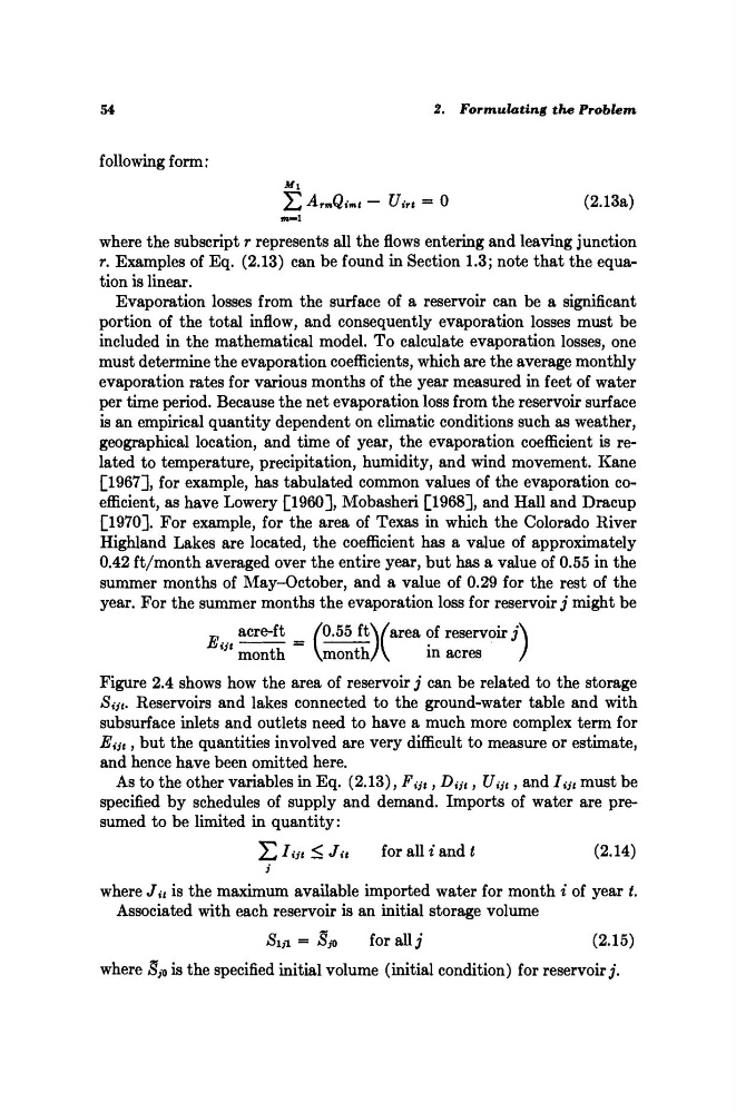
year. For the summer months the evaporation loss for reservoir j might be
acre-ft _ /0.55 ft\/area of reservoir A
%Jt month
\month/\
in acres
/
Figure 2.4 shows how the area of reservoir j can be related to the storage
Sij t .
Reservoirs and lakes connected to the ground-water table and with
subsurface inlets and outlets need to have a much more complex term for
Εφ > but the quantities involved are very difficult to measure or estimate,
and hence have been omitted here.
As to the other variables in Eq. (2.13), Εφ , Όφ , ϋφ , and Iφ must be
specified by schedules of supply and demand. Imports of water are presumed to be limited in quantity:
ΣIm ^ Ju
ioT a11 i
a n d
*
(2.14)
i
where Ju is the maximum available imported water for month i of year t.
Associated with each reservoir is an initial storage volume
S w = Β jo
for allj
(2.15)
where Sjo is the specified initial volume (initial condition) for reservoir j.
2. Formulating
the Problem
following form:
Mi
Σ A rm Q imt
- U irt = 0
(2.13a)
where the subscript r represents all the flows entering and leaving junction
r. Examples of Eq. (2.13) can be found in Section 1.3; note that the equation is linear.
Evaporation losses from the surface of a reservoir can be a significant
portion of the total inflow, and consequently evaporation losses must be
included in the mathematical model. To calculate evaporation losses, one
must determine the evaporation coefficients, which are the average monthly
evaporation rates for various months of the year measured in feet of water
per time period. Because the net evaporation loss from the reservoir surface
is an empirical quantity dependent on climatic conditions such as weather,
geographical location, and time of year, the evaporation coefficient is related to temperature, precipitation, humidity, and wind movement. Kane
[1967], for example, has tabulated common values of the evaporation coefficient, as have Lowery [1960], Mobasheri [1968], and Hall and Dracup
[1970]. For example, for the area of Texas in which the Colorado River
Highland Lakes are located, the coefficient has a value of approximately
0.42 ft/month averaged over the entire year, but has a value of 0.55 in the
summer months of May-October, and a value of 0.29 for the rest of the
year. For the summer months the evaporation loss for reservoir j might be
acre-ft _ /0.55 ft\/area of reservoir A
%Jt month
\month/\
in acres
/
Figure 2.4 shows how the area of reservoir j can be related to the storage
Sij t .
Reservoirs and lakes connected to the ground-water table and with
subsurface inlets and outlets need to have a much more complex term for
Εφ > but the quantities involved are very difficult to measure or estimate,
and hence have been omitted here.
As to the other variables in Eq. (2.13), Εφ , Όφ , ϋφ , and Iφ must be
specified by schedules of supply and demand. Imports of water are presumed to be limited in quantity:
ΣIm ^ Ju
ioT a11 i
a n d
*
(2.14)
i
where Ju is the maximum available imported water for month i of year t.
Associated with each reservoir is an initial storage volume
S w = Β jo
for allj
(2.15)
where Sjo is the specified initial volume (initial condition) for reservoir j.