

2.3.
Constraints
43
impact on the optimum design is small while their contribution to the
mathematical complexity is large. Other variables that are continuous,
such as the river flow, have to be treated as discrete. However, it is believed that the model developed here is a reasonably accurate representation of a multipurpose water resources system and contains the variables
that are the most relevant for optimal planning.
2.3.1. Budgetary
Constraints
The capital budgetary constraint is calculated differently in the private
and public sectors. In the private sector it is considered to be a function
of a corporation's current assets and current debt level. In the public
sector it is dependent upon congressional or state water resources appropriations. While it is clear that constraints on capital spending exist, the quantitative formulation of such constraints is quite subjective. Here we will
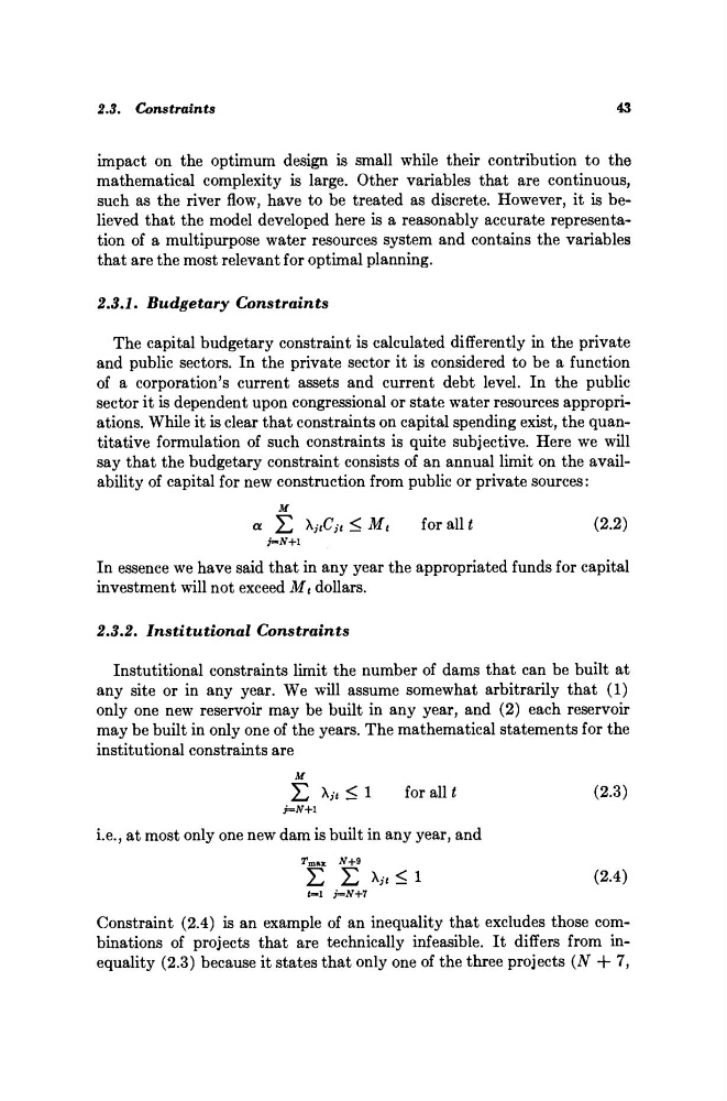
say that the budgetary constraint consists of an annual limit on the availability of capital for new construction from public or private sources:
Μ
α Σ Xy f Cy< < M t
for all t
(2.2)
In essence we have said that in any year the appropriated funds for capital
investment will not exceed M t dollars.
2.3.2. Institutional
Constraints
Instutitional constraints limit the number of dams that can be built at
any site or in any year. We w
r ill assume somewhat arbitrarily that (1)
only one new reservoir may be built in any year, and (2) each reservoir
may be built in only one of the years. The mathematical statements for the
institutional constraints are
Μ
Σ λ;< < 1 for all t
(2.3)
i.e., at most only one new dam is built in any year, and
TmAX
ΛΓ+9
Σ Σ λ* < 1
(2.4)
ί=1
j=N+7
Constraint (2.4) is an example of an inequality that excludes those combinations of projects that are technically infeasible. It differs from inequality (2.3) because it states that only one of the three projects (N + 7,
Constraints
43
impact on the optimum design is small while their contribution to the
mathematical complexity is large. Other variables that are continuous,
such as the river flow, have to be treated as discrete. However, it is believed that the model developed here is a reasonably accurate representation of a multipurpose water resources system and contains the variables
that are the most relevant for optimal planning.
2.3.1. Budgetary
Constraints
The capital budgetary constraint is calculated differently in the private
and public sectors. In the private sector it is considered to be a function
of a corporation's current assets and current debt level. In the public
sector it is dependent upon congressional or state water resources appropriations. While it is clear that constraints on capital spending exist, the quantitative formulation of such constraints is quite subjective. Here we will
say that the budgetary constraint consists of an annual limit on the availability of capital for new construction from public or private sources:
Μ
α Σ Xy f Cy< < M t
for all t
(2.2)
In essence we have said that in any year the appropriated funds for capital
investment will not exceed M t dollars.
2.3.2. Institutional
Constraints
Instutitional constraints limit the number of dams that can be built at
any site or in any year. We w
r ill assume somewhat arbitrarily that (1)
only one new reservoir may be built in any year, and (2) each reservoir
may be built in only one of the years. The mathematical statements for the
institutional constraints are
Μ
Σ λ;< < 1 for all t
(2.3)
i.e., at most only one new dam is built in any year, and
TmAX
ΛΓ+9
Σ Σ λ* < 1
(2.4)
ί=1
j=N+7
Constraint (2.4) is an example of an inequality that excludes those combinations of projects that are technically infeasible. It differs from inequality (2.3) because it states that only one of the three projects (N + 7,