

1.3. Techniques for the Optimization
of a Water Resources
System
25
benefits can be expressed by
recreation revenue = c jt — dj t [Ej t
— Sji]
2
where Cj t and dj t are known constants and E Jt is the optimal amount of
water in the reservoir. Then the objective function to be maximized would
be
Jmax
3
/(*) = ΣΣ
oc{a it D% + b jt D jt + c jt - d,lE Jt
-
S jt J}
where a is the discount factor that reduces all dollars to their present
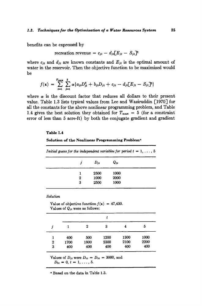
value. Table 1.3 lists typical values from Lee and Waziruddin [1970] for
all the constants for the above nonlinear programming problem, and Table
1.4 gives the best solution they obtained for T max = 5 (for a constraint
error of less than 5 acre-ft) by both the conjugate gradient and gradient
Table 1.4
Solution of the Nonlinear Programming Problem
0
Initial guess for the independent variables for period t = 1, ..., 5
1
2500
1000
2
1000
2000
3
2500
1000
Solution
Value of objective function/(x) = 47,430.
Values of Qj t were as follows:
t
3
1
2
3
4
5
1
400
500
1200
1300
1000
2
1700
1800
2300
2100
2200
3
400
400
400
400
400
Values of D it were D u = D zt = 3000, and
D 2t = 0, t = 1, ..., 5.
a
Based on the data in Table 1.3.
of a Water Resources
System
25
benefits can be expressed by
recreation revenue = c jt — dj t [Ej t
— Sji]
2
where Cj t and dj t are known constants and E Jt is the optimal amount of
water in the reservoir. Then the objective function to be maximized would
be
Jmax
3
/(*) = ΣΣ
oc{a it D% + b jt D jt + c jt - d,lE Jt
-
S jt J}
where a is the discount factor that reduces all dollars to their present
value. Table 1.3 lists typical values from Lee and Waziruddin [1970] for
all the constants for the above nonlinear programming problem, and Table
1.4 gives the best solution they obtained for T max = 5 (for a constraint
error of less than 5 acre-ft) by both the conjugate gradient and gradient
Table 1.4
Solution of the Nonlinear Programming Problem
0
Initial guess for the independent variables for period t = 1, ..., 5
1
2500
1000
2
1000
2000
3
2500
1000
Solution
Value of objective function/(x) = 47,430.
Values of Qj t were as follows:
t
3
1
2
3
4
5
1
400
500
1200
1300
1000
2
1700
1800
2300
2100
2200
3
400
400
400
400
400
Values of D it were D u = D zt = 3000, and
D 2t = 0, t = 1, ..., 5.
a
Based on the data in Table 1.3.