

6.3. Formulating
the Problem to Include Water
Quality
151
i.e., at most only one new treatment plant is built in any year. Also,
Tmax JV*+12
Σ Σ Xyi < 1
(6.4)
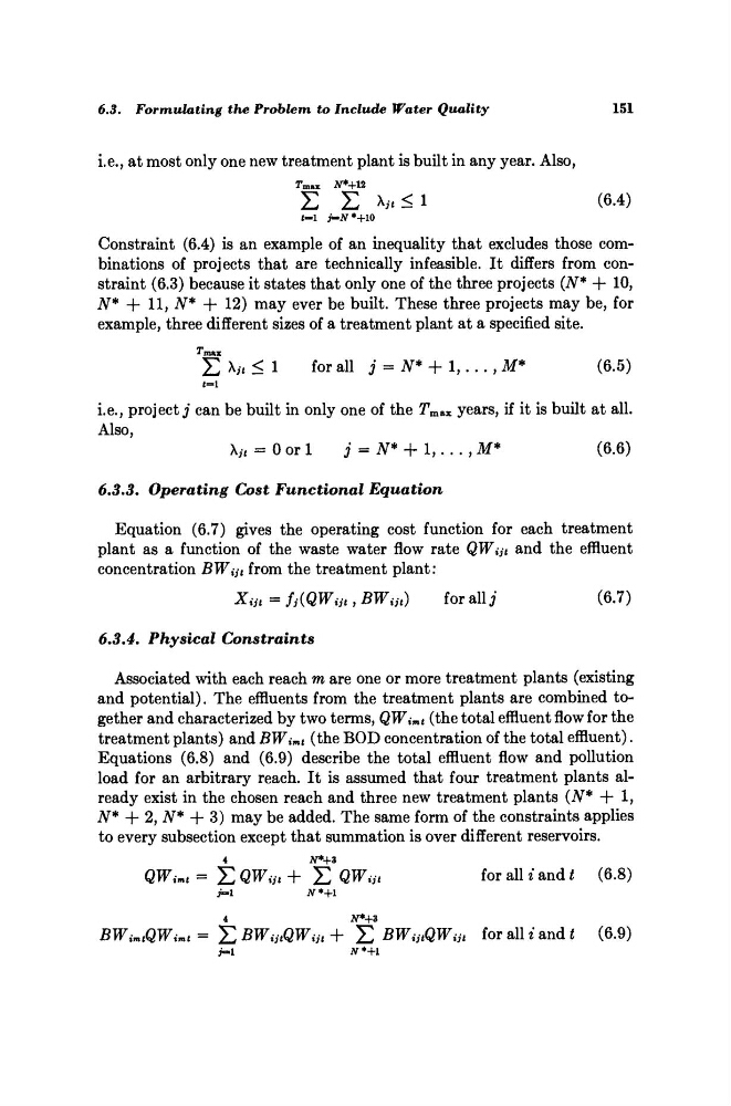
Constraint (6.4) is an example of an inequality that excludes those combinations of projects that are technically infeasible. It differs from constraint (6.3) because it states that only one of the three projects (ΛΓ* + 10,
N* + 11, N* + 12) may ever be built. These three projects may be, for
example, three different sizes of a treatment plant at a specified site.
Σ X y< < 1
for all j = N* + 1,..., M*
(6.5)
i.e., project j can be built in only one of the T mM years, if it is built at all.
Also,
X jt = 0 or 1
j = iV* + 1,.. ., M*
(6.6)
6.3.3. Operating
Cost Functional
Equation
Equation (6.7) gives the operating cost function for each treatment
plant as a function of the waste water flow rate QWi Jt
and the effluent
concentration BWijt from the treatment plant:
Xijt = fj(QW ijt ,
BWijt)
for allj
(6.7)
6.3.4. Physical
Constraints
Associated with each reach m are one or more treatment plants (existing
and potential). The effluents from the treatment plants are combined together and characterized by two terms, QWimt (the total effluent flow for the
treatment plants) and BWi mt
(the BOD concentration of the total effluent).
Equations (6.8) and (6.9) describe the total effluent flow and pollution
load for an arbitrary reach. It is assumed that four treatment plants already exist in the chosen reach and three new treatment plants (iV* + 1,
iV* + 2, N* + 3) may be added. The same form of the constraints applies
to every subsection except that summation is over different reservoirs.
4
N*+3
QW^t
= Σ QWijt
+
Σ
QWijt
for all i and t
(6.8)
4
ΛΓ*+3
BW imt QWi mt
= T*BWijtQWij t +
Y.BWijtQWijt
for all i and t
(6.9)
the Problem to Include Water
Quality
151
i.e., at most only one new treatment plant is built in any year. Also,
Tmax JV*+12
Σ Σ Xyi < 1
(6.4)
Constraint (6.4) is an example of an inequality that excludes those combinations of projects that are technically infeasible. It differs from constraint (6.3) because it states that only one of the three projects (ΛΓ* + 10,
N* + 11, N* + 12) may ever be built. These three projects may be, for
example, three different sizes of a treatment plant at a specified site.
Σ X y< < 1
for all j = N* + 1,..., M*
(6.5)
i.e., project j can be built in only one of the T mM years, if it is built at all.
Also,
X jt = 0 or 1
j = iV* + 1,.. ., M*
(6.6)
6.3.3. Operating
Cost Functional
Equation
Equation (6.7) gives the operating cost function for each treatment
plant as a function of the waste water flow rate QWi Jt
and the effluent
concentration BWijt from the treatment plant:
Xijt = fj(QW ijt ,
BWijt)
for allj
(6.7)
6.3.4. Physical
Constraints
Associated with each reach m are one or more treatment plants (existing
and potential). The effluents from the treatment plants are combined together and characterized by two terms, QWimt (the total effluent flow for the
treatment plants) and BWi mt
(the BOD concentration of the total effluent).
Equations (6.8) and (6.9) describe the total effluent flow and pollution
load for an arbitrary reach. It is assumed that four treatment plants already exist in the chosen reach and three new treatment plants (iV* + 1,
iV* + 2, N* + 3) may be added. The same form of the constraints applies
to every subsection except that summation is over different reservoirs.
4
N*+3
QW^t
= Σ QWijt
+
Σ
QWijt
for all i and t
(6.8)
4
ΛΓ*+3
BW imt QWi mt
= T*BWijtQWij t +
Y.BWijtQWijt
for all i and t
(6.9)