

128
4. Application of the Optimization
Algorithm
BOUND is called once by the main program for each year. The running
time for BOUND is greatest in the earlier years (when the number of
possible choices is greatest) and then decreases accordingly as reservoirs
are built, thereby reducing the number of choices for succeeding years.
In the example described above, a library subroutine of the CDC 6600
computation system (subroutine SECOND) was used to isolate the calculation time for subroutines OLERSEN and BOUND. For 50 years of calculations, subroutine OLERSEN was called 53 times for a total computing
time of 3.735 sec; individual computing times ranged from 0.112 to 0.044
sec. Subroutine BOUND was called 50 times for a total computing time
of 2.099 sec; individual computing times ranged from 0.238 to 0.019 sec.
The combined computing time for all calculations in subroutines OLERSEN and BOUND was 5.824 sec, which was approximately 95% of the
total computing time needed to obtain a first feasible solution (6.138 sec).
For a problem having a different network configuration, the following
steps are needed to estimate the computation time needed to find a first
feasible solution:
1. Use routine OLERSEN as a main program and empirically find its
running time (*OLER) with the problem network configuration as data. Use
different sets of perturbed data to get an average running time. Estimate
the number of times OLERSEN will be called by the main program
(N OLER) .
2. Determine the running time for BOUND (UBXO)
for different
combinations of possible reservoir choices. Estimate the number of years
each combination of projects is under consideration (F»BND).
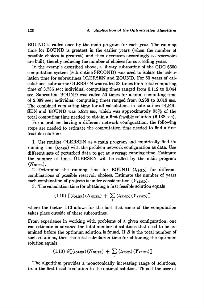
3. The calculation time for obtaining a first feasible solution equals
(1.10) £(£OLER) (NOLER) + Σ (*;BND)(I^BND)]
where the factor 1.10 allows for the fact that some of the computation
takes place outside of these subroutines.
From experience in working with problems of a given configuration, one
can estimate in advance the total number of solutions that need to be examined before the optimum solution, is found. If S is the total number of
such solutions, then the total calculation time for obtaining the optimum
solution equals
(1.10) £[(< 0 LER) (#OLER) + Σ (^BNDKF.BND)]
t
The algorithm provides a monotonically increasing range of solutions,
from the first feasible solution to the optimal solution. Thus if the user of
4. Application of the Optimization
Algorithm
BOUND is called once by the main program for each year. The running
time for BOUND is greatest in the earlier years (when the number of
possible choices is greatest) and then decreases accordingly as reservoirs
are built, thereby reducing the number of choices for succeeding years.
In the example described above, a library subroutine of the CDC 6600
computation system (subroutine SECOND) was used to isolate the calculation time for subroutines OLERSEN and BOUND. For 50 years of calculations, subroutine OLERSEN was called 53 times for a total computing
time of 3.735 sec; individual computing times ranged from 0.112 to 0.044
sec. Subroutine BOUND was called 50 times for a total computing time
of 2.099 sec; individual computing times ranged from 0.238 to 0.019 sec.
The combined computing time for all calculations in subroutines OLERSEN and BOUND was 5.824 sec, which was approximately 95% of the
total computing time needed to obtain a first feasible solution (6.138 sec).
For a problem having a different network configuration, the following
steps are needed to estimate the computation time needed to find a first
feasible solution:
1. Use routine OLERSEN as a main program and empirically find its
running time (*OLER) with the problem network configuration as data. Use
different sets of perturbed data to get an average running time. Estimate
the number of times OLERSEN will be called by the main program
(N OLER) .
2. Determine the running time for BOUND (UBXO)
for different
combinations of possible reservoir choices. Estimate the number of years
each combination of projects is under consideration (F»BND).
3. The calculation time for obtaining a first feasible solution equals
(1.10) £(£OLER) (NOLER) + Σ (*;BND)(I^BND)]
where the factor 1.10 allows for the fact that some of the computation
takes place outside of these subroutines.
From experience in working with problems of a given configuration, one
can estimate in advance the total number of solutions that need to be examined before the optimum solution, is found. If S is the total number of
such solutions, then the total calculation time for obtaining the optimum
solution equals
(1.10) £[(< 0 LER) (#OLER) + Σ (^BNDKF.BND)]
t
The algorithm provides a monotonically increasing range of solutions,
from the first feasible solution to the optimal solution. Thus if the user of