

118
4. Application
of the Optimization
Algorithm
+
Σ
a
(6ΐ3,12/ΐ3,12 + 6δ3,52/63,62)
f-l
net operating return from the newly
added subsystems
7max
- Σ a Χ 10
6 [λ Μ (40.0) + λ 7ι< (6.3) + · · · + λι Μ (5.55)]
*-l
capital cost of the projects over the planning period
The λ values are determined by the optimization algorithm. Table 4.5a
lists the cost coefficients 6.7 for the first term, Table 4.3 lists those for the
second term, and Table 4.1 lists those for the third term. Arcs with nonzero
cost coefficients will be referred to as NZC arcs.
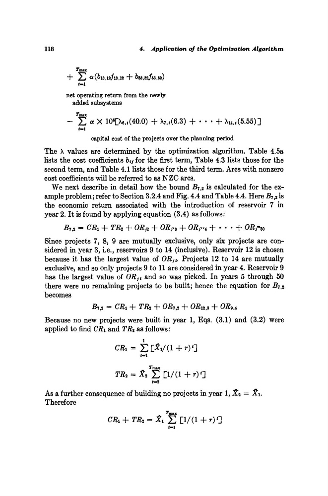
We next describe in detail how the bound #7,2 is calculated for the example problem; refer to Section 3.2.4 and Fig. 4.4 and Table 4.4. Here £7,2 is
the economic return associated with the introduction of reservoir 7 in
year 2. It is found by applying equation (3.4) as follows:
£7,2 =
CRi +
TR * +
0 R v + 0R 3'* +
0R i"i + · · · + OR,**
Since projects 7, 8, 9 are mutually exclusive, only six projects are considered in year 3, i.e., reservoirs 9 to 14 (inclusive). Reservoir 12 is chosen
because it has the largest value of 0R Jt . Projects 12 to 14 are mutually
exclusive, and so only projects 9 to 11 are considered in year 4. Reservoir 9
has the largest value of 0R 3t and so was picked. In years 5 through 50
there were no remaining projects to be built; hence the equation for J?7,2
becomes
-67,2 =
CRi + TR2 "H ORi t 2 -F- OJ?i2,3 "F~ OR94
Because no new projects were built in year 1, Eqs. (3.1) and (3.2) were
applied to find CRi and TR* as follows:
CR X =
E[£i/(l + r)<]
t-i
<-2
As a further consequence of building no projects in year 1, 3t 2 = £1.
Therefore
CRi + TR 2 - ί
[1/(1 + r)<]
1-1
4. Application
of the Optimization
Algorithm
+
Σ
a
(6ΐ3,12/ΐ3,12 + 6δ3,52/63,62)
f-l
net operating return from the newly
added subsystems
7max
- Σ a Χ 10
6 [λ Μ (40.0) + λ 7ι< (6.3) + · · · + λι Μ (5.55)]
*-l
capital cost of the projects over the planning period
The λ values are determined by the optimization algorithm. Table 4.5a
lists the cost coefficients 6.7 for the first term, Table 4.3 lists those for the
second term, and Table 4.1 lists those for the third term. Arcs with nonzero
cost coefficients will be referred to as NZC arcs.
We next describe in detail how the bound #7,2 is calculated for the example problem; refer to Section 3.2.4 and Fig. 4.4 and Table 4.4. Here £7,2 is
the economic return associated with the introduction of reservoir 7 in
year 2. It is found by applying equation (3.4) as follows:
£7,2 =
CRi +
TR * +
0 R v + 0R 3'* +
0R i"i + · · · + OR,**
Since projects 7, 8, 9 are mutually exclusive, only six projects are considered in year 3, i.e., reservoirs 9 to 14 (inclusive). Reservoir 12 is chosen
because it has the largest value of 0R Jt . Projects 12 to 14 are mutually
exclusive, and so only projects 9 to 11 are considered in year 4. Reservoir 9
has the largest value of 0R 3t and so was picked. In years 5 through 50
there were no remaining projects to be built; hence the equation for J?7,2
becomes
-67,2 =
CRi + TR2 "H ORi t 2 -F- OJ?i2,3 "F~ OR94
Because no new projects were built in year 1, Eqs. (3.1) and (3.2) were
applied to find CRi and TR* as follows:
CR X =
E[£i/(l + r)<]
t-i
<-2
As a further consequence of building no projects in year 1, 3t 2 = £1.
Therefore
CRi + TR 2 - ί
[1/(1 + r)<]
1-1