

3.4. Application
of the OKA to the Operational
Policy
Problem
103
If it is assumed that each turbine operates at a constant head and at a
constant speed, there is a linear relationship between flow and energy.
In the example water resources problem (fully described in Chapter 4)
the OKA is repeatedly applied to solve the OP problem. Sections 4.2
and 4.3 describe how the OKA optimizes the flow variables of the original
system network whose configuration is detailed in Tables B.3 and B.4.
The solution procedure followed is identical to that described in Sections
3.3.1-3.3.7 and utilized in Section 3.3.8. However, the complexity of the
problem precludes the listing of intermediate results.
START
I INITIALIZE ALL VARIABLES
READ DATA:
(A) SIZE AND COST (CAPITAL AND
OPERATING) OF EACH RESERVOIR
(B) SPATIAL CONFIGURATION OF THE
NETWORK
(C) UPPER AND LOWER FLOW
CAPACITIES OF EACH ARC
(D) COST OF PASSING ONE UNIT OF
FLOW THROUGH EACH ARC
CALCULATE THE PRESENT VALUE
FOR EACH NEW PROJECT AND YEAR OR jT
CALCULATE AVAILABLE CAPITAL AND
SYSTEM DEMANDS (e
IRRIGATION
AND POWER)
DETERMINE FEASIBLE ALTERNATIVES
CALCULATE
FOR THESE ALTERNATIVES
SELECT MAXIMUM Β ω. „(«' >
r(i')i
CALCULATE X^' ANDX V / ' (ONE-YEAR
OPTIMIZATION PROBLEM)
BRANCH TOt"
CHANGE UPPER BOUND
FOR RESERVOIR V IN
THE NETWORK
BRANCH TO 0
NO PROJECT IS BUILT
PRINT CUMULATIVE RETURN
FOR ALL PERIODS TO PERIOD Τ
NO
<Γ^^ Τ <
YES YES
WE HAVE A FIRST FEASIBLE
SOLUTION PVERN (i", Tmax)
GO TO PART 2 OF
THE ALGORITHM
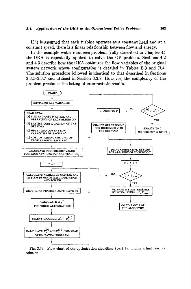
Fig. 3.14 Flow chart of the optimization algorithm (part 1): finding a first feasible
solution.
of the OKA to the Operational
Policy
Problem
103
If it is assumed that each turbine operates at a constant head and at a
constant speed, there is a linear relationship between flow and energy.
In the example water resources problem (fully described in Chapter 4)
the OKA is repeatedly applied to solve the OP problem. Sections 4.2
and 4.3 describe how the OKA optimizes the flow variables of the original
system network whose configuration is detailed in Tables B.3 and B.4.
The solution procedure followed is identical to that described in Sections
3.3.1-3.3.7 and utilized in Section 3.3.8. However, the complexity of the
problem precludes the listing of intermediate results.
START
I INITIALIZE ALL VARIABLES
READ DATA:
(A) SIZE AND COST (CAPITAL AND
OPERATING) OF EACH RESERVOIR
(B) SPATIAL CONFIGURATION OF THE
NETWORK
(C) UPPER AND LOWER FLOW
CAPACITIES OF EACH ARC
(D) COST OF PASSING ONE UNIT OF
FLOW THROUGH EACH ARC
CALCULATE THE PRESENT VALUE
FOR EACH NEW PROJECT AND YEAR OR jT
CALCULATE AVAILABLE CAPITAL AND
SYSTEM DEMANDS (e
IRRIGATION
AND POWER)
DETERMINE FEASIBLE ALTERNATIVES
CALCULATE
FOR THESE ALTERNATIVES
SELECT MAXIMUM Β ω. „(«' >
r(i')i
CALCULATE X^' ANDX V / ' (ONE-YEAR
OPTIMIZATION PROBLEM)
BRANCH TOt"
CHANGE UPPER BOUND
FOR RESERVOIR V IN
THE NETWORK
BRANCH TO 0
NO PROJECT IS BUILT
PRINT CUMULATIVE RETURN
FOR ALL PERIODS TO PERIOD Τ
NO
<Γ^^ Τ <
YES YES
WE HAVE A FIRST FEASIBLE
SOLUTION PVERN (i", Tmax)
GO TO PART 2 OF
THE ALGORITHM
Fig. 3.14 Flow chart of the optimization algorithm (part 1): finding a first feasible
solution.