

44
STANLEY CORRSIN
vary considerably over distances comparable to the leqth scales characterizing the ’L eddies.”
As a more recent illustration, we can we the turbulent boundary layer
data of Blackwelder and Kovasznay (1972), by astimating a length characteristic of momentum transport. A plausible choice would be the product of
Lagrangian integral time scale of turbulent velocity and rms value of the
same velocity. Unfortunately, there are no data available on Lagrangian
velocity autocorrelation function in any of tbc traditional turbulent shear
flows, but we might speculate that the Eulerian integral time scale in a frame
convected downstream at the s p e d for maximum correlation at each distance will be the same order of magnitude as the Lagrangian time scale (the
isotropic case has been studied: Cornin, 1963; Shlien and Corrsin, 1974).
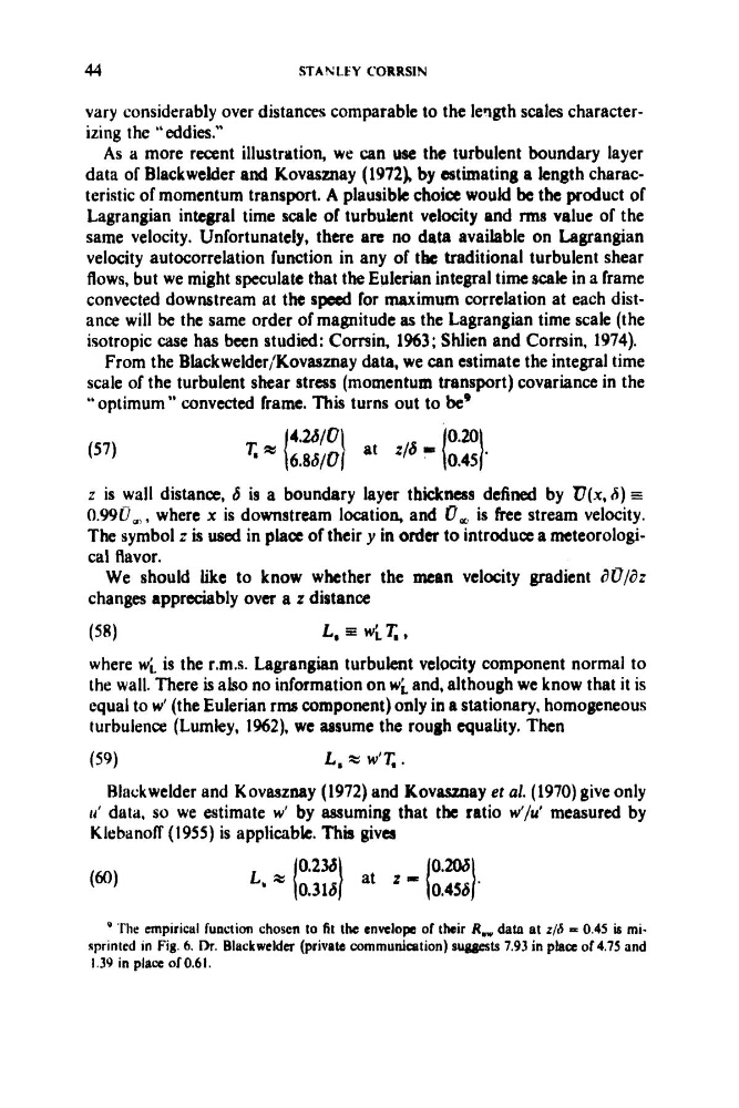
From the Blackwelder/Kovasznay data, we can estimate the integral time
scale of the turbulent shear stress (momentum transport) covariance in the
“optimum” convected frame. This turns out to be9
(57)
z is wall distance, 6 is a boundary layer thickness defined by D(x, S) =
0.9917,,, where x is downstream location, and 0, is h e stream velocity.
The symbol z is used in place of their y in order to introduce a meteorological flavor.
We should like to know whether the mean velocity gradient dO/az
changes appreciably over a z distance
(58)
L, W i T , ,
where w i is the r.m.s. Lagrangian turbulent velocity component normal to
the wall. There is also no information on wt and, although we know that it is
equal to w’ (the Eulerian rms component) only in a stationary, homogeneous
turbulence (Lumley, 1962). we assume the rough equality. Then
(59)
t, 4 W I T , ,
Blackwelder and Kovasznay (1972) and Kovasznay et al. (1970) give only
11’ data, so we estimate w’ by assuming that thc ratio w‘/d measured by
Klebanoff (1955) is appiicabk. This gives
0.236
0.206
Ln (0.316) at = (0.456).
’ The empiricul function chosen to fit the envelop of their R,, data at 2/15 = 0.45 is misprinted in Fig. 6. Dr. Bluckwelda (private communication) suggests 7.93 in place of 4.75 and
1.39 in place of 0.61.
STANLEY CORRSIN
vary considerably over distances comparable to the leqth scales characterizing the ’L eddies.”
As a more recent illustration, we can we the turbulent boundary layer
data of Blackwelder and Kovasznay (1972), by astimating a length characteristic of momentum transport. A plausible choice would be the product of
Lagrangian integral time scale of turbulent velocity and rms value of the
same velocity. Unfortunately, there are no data available on Lagrangian
velocity autocorrelation function in any of tbc traditional turbulent shear
flows, but we might speculate that the Eulerian integral time scale in a frame
convected downstream at the s p e d for maximum correlation at each distance will be the same order of magnitude as the Lagrangian time scale (the
isotropic case has been studied: Cornin, 1963; Shlien and Corrsin, 1974).
From the Blackwelder/Kovasznay data, we can estimate the integral time
scale of the turbulent shear stress (momentum transport) covariance in the
“optimum” convected frame. This turns out to be9
(57)
z is wall distance, 6 is a boundary layer thickness defined by D(x, S) =
0.9917,,, where x is downstream location, and 0, is h e stream velocity.
The symbol z is used in place of their y in order to introduce a meteorological flavor.
We should like to know whether the mean velocity gradient dO/az
changes appreciably over a z distance
(58)
L, W i T , ,
where w i is the r.m.s. Lagrangian turbulent velocity component normal to
the wall. There is also no information on wt and, although we know that it is
equal to w’ (the Eulerian rms component) only in a stationary, homogeneous
turbulence (Lumley, 1962). we assume the rough equality. Then
(59)
t, 4 W I T , ,
Blackwelder and Kovasznay (1972) and Kovasznay et al. (1970) give only
11’ data, so we estimate w’ by assuming that thc ratio w‘/d measured by
Klebanoff (1955) is appiicabk. This gives
0.236
0.206
Ln (0.316) at = (0.456).
’ The empiricul function chosen to fit the envelop of their R,, data at 2/15 = 0.45 is misprinted in Fig. 6. Dr. Bluckwelda (private communication) suggests 7.93 in place of 4.75 and
1.39 in place of 0.61.