

NUMERICAL COMPUTATION OF TLlRRCrLENT SHEAR FI.OWS
23 I
No-slip boundaries are best treated by Chebyshev expansion in x3
(Orszag. 1971b). The velocity field is represented as
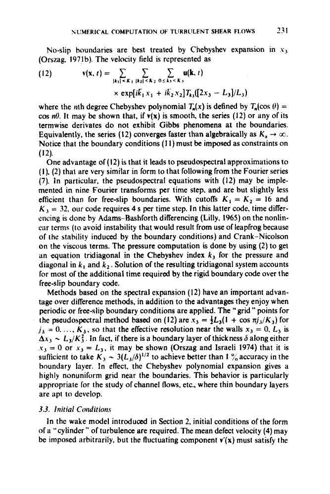
V(X, t ) = 1 C C u(k, I )
I k i I < E l l I k z I < A z O S k r < A i
(12)
x exp[ik,x, + i ~ , . ~ ~ ] 7 # . ~ ~
- L 3 ] / L 3 )
where the nth degree Chebyshev polynomial T,(x) is defined by T,(cos 0) =
cos nu. It may be shown that, if v(x) is smooth, the series (12) or any of its
termwise derivates do not exhibit Gibbs phenomena at the boundaries.
Equivalently, the series (12) converges faster than algebraically as K, --* cc.
Notice that the boundary conditions (1 1) must be imposed as constraints on
One advantage of (12) is that it leads to pseudospectral approximations to
(I), (2) that are very similar in form to that following from the Fourier series
(7). In particular, the pseudospectral equations with (12) may be implemented in nine Fourier transforms per time step, and are but slightly less
efficient than for free-slip boundaries. With cutoffs K , = K 2 = 16 and
K 3 = 32, our code requires 4 s per time step. In this latter code, time differencing is done by Adams-Bashforth differencing (Lilly, 1965) on the nonlinear terms (to avoid instability that would result from use of leapfrog because
of the stability induced by the boundary conditions) and Crank-Nicolson
on the viscous terms. The pressure computation is done by using (2) to get
an equation tridiagonal in the Chebyshev index k3 for the pressure and
diagonal in k l and k2. Solution of the resulting tridiagonal system accounts
for most of the additional time required by the rigid boundary code over the
free-slip boundary code.
Methods based on the spectral expansion (12) have an important advantage over difference methods, in addition to the advantages they enjoy when
periodic or free-slip boundary conditions are applied. The “grid ” points for
the pseudospectral method based on (12) are x3 = fL,(l + cos 7rj.3/K3) for
j 3 = 0. . . ., K 3 . so that the effective resolution near the walls x3 = 0. L3 is
Ax3 - L , / K : . In fact, if there is a boundary layer of thickness 6 along either
Y., = 0 or x3 = I-.,, it may be shown (Orszag and Israeli 1974) that it is
sufficient to take K, - 3(L3/41’2 to achieve better than 1 ”/accuracy in the
boundary layer. In effect, the Chebyshev polynomial expansion gives a
highly nonuniform grid near the boundaries. This behavior is particularly
appropriate for the study of channel flows, etc., where thin boundary layers
are apt to develop.
3.3. Initial Conditions
In the wake model introduced in Section 2, initial conditions of the form
of a ”cylinder ” of turbulence are required. The mean defect velocity (4) may
be imposed arbitrarily, but the fluctuating component v’(x) must satisfy the
(12).
23 I
No-slip boundaries are best treated by Chebyshev expansion in x3
(Orszag. 1971b). The velocity field is represented as
V(X, t ) = 1 C C u(k, I )
I k i I < E l l I k z I < A z O S k r < A i
(12)
x exp[ik,x, + i ~ , . ~ ~ ] 7 # . ~ ~
- L 3 ] / L 3 )
where the nth degree Chebyshev polynomial T,(x) is defined by T,(cos 0) =
cos nu. It may be shown that, if v(x) is smooth, the series (12) or any of its
termwise derivates do not exhibit Gibbs phenomena at the boundaries.
Equivalently, the series (12) converges faster than algebraically as K, --* cc.
Notice that the boundary conditions (1 1) must be imposed as constraints on
One advantage of (12) is that it leads to pseudospectral approximations to
(I), (2) that are very similar in form to that following from the Fourier series
(7). In particular, the pseudospectral equations with (12) may be implemented in nine Fourier transforms per time step, and are but slightly less
efficient than for free-slip boundaries. With cutoffs K , = K 2 = 16 and
K 3 = 32, our code requires 4 s per time step. In this latter code, time differencing is done by Adams-Bashforth differencing (Lilly, 1965) on the nonlinear terms (to avoid instability that would result from use of leapfrog because
of the stability induced by the boundary conditions) and Crank-Nicolson
on the viscous terms. The pressure computation is done by using (2) to get
an equation tridiagonal in the Chebyshev index k3 for the pressure and
diagonal in k l and k2. Solution of the resulting tridiagonal system accounts
for most of the additional time required by the rigid boundary code over the
free-slip boundary code.
Methods based on the spectral expansion (12) have an important advantage over difference methods, in addition to the advantages they enjoy when
periodic or free-slip boundary conditions are applied. The “grid ” points for
the pseudospectral method based on (12) are x3 = fL,(l + cos 7rj.3/K3) for
j 3 = 0. . . ., K 3 . so that the effective resolution near the walls x3 = 0. L3 is
Ax3 - L , / K : . In fact, if there is a boundary layer of thickness 6 along either
Y., = 0 or x3 = I-.,, it may be shown (Orszag and Israeli 1974) that it is
sufficient to take K, - 3(L3/41’2 to achieve better than 1 ”/accuracy in the
boundary layer. In effect, the Chebyshev polynomial expansion gives a
highly nonuniform grid near the boundaries. This behavior is particularly
appropriate for the study of channel flows, etc., where thin boundary layers
are apt to develop.
3.3. Initial Conditions
In the wake model introduced in Section 2, initial conditions of the form
of a ”cylinder ” of turbulence are required. The mean defect velocity (4) may
be imposed arbitrarily, but the fluctuating component v’(x) must satisfy the
(12).