

216
P. J. S1II.LIVAN
one may expect the average value of r and the Eulerian integral length scale
of turbulence in the cross strcam direction to be comparable. The numbers
along the typical trajectory shown in Fig. 1 refer to the number of time
intervals from the start of the record. These figures suggest that one radius of
curvature may well describe the trajectory over quite a large number of time
intervals.
2. LENGTH SCALES
The particle trajectories are smoothed to reduce the small scale erratic
behaviour resulting from experimental error in spatial and temporal resolution and perhaps resulting from scales of turbulence far into dissipation
range of sizes. In each trajectory the values of adjacent coordinate positions
are averaged, i.e., z, = (zi + zi+ ,)/2 and yj = (yi + y I + ,)/2, and this is
repeated 20 times for each record. Figure 1 with n = 10 and n = 20 shows
the change in the trajectory for 10 and 20 repetitions of the averaging
procedure. The smoothed trajectories with n = 20 are used for further statistical information.
The channel depth is subdivided into 10 equal segments on z. Using
experimental values that are found in each of these 10 horizontal slabs an
experimental probability density function p(r’) is compiled. Figures 2a and
2b show the experimental data and the solid curve on these figures is calculated from
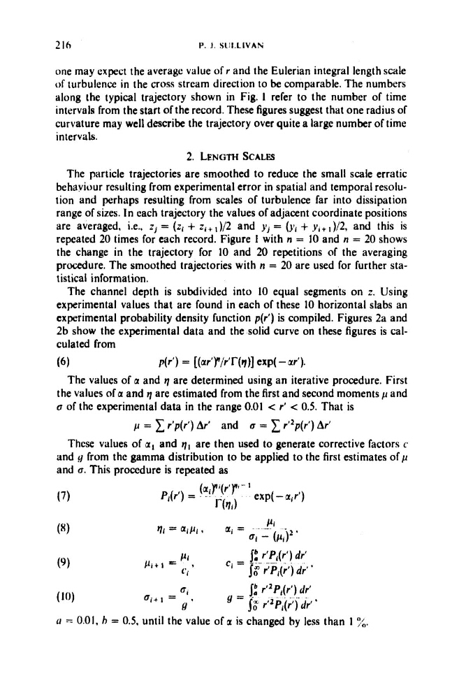
(6)
p(r’) = [(ar’p/rT(q)] expj -ar’).
The values of a and g are determined using an iterative procedure. First
the values of a and g are estimated from the first and second moments p and
cr of the experimental data in the range 0.01 < r’ < 0.5. That is
p = r’p(r’) Ar’ and 0 = r’*p(r’) Ar’
These values of a1 and ql are then used to generate corrective factors c‘
and 11 from the gamma distribution to be applied to the first estimates of p
and cr. This procedure is repeated as
(7)
1.” r‘P.(r’) dr’
J$ r‘Pi(r’) dr’ ’
Pi
c , = -. - --!
P i + l = ci.
u - 1 0.01, h = 0.5, until the value of a is changed by less than 1 x.
P. J. S1II.LIVAN
one may expect the average value of r and the Eulerian integral length scale
of turbulence in the cross strcam direction to be comparable. The numbers
along the typical trajectory shown in Fig. 1 refer to the number of time
intervals from the start of the record. These figures suggest that one radius of
curvature may well describe the trajectory over quite a large number of time
intervals.
2. LENGTH SCALES
The particle trajectories are smoothed to reduce the small scale erratic
behaviour resulting from experimental error in spatial and temporal resolution and perhaps resulting from scales of turbulence far into dissipation
range of sizes. In each trajectory the values of adjacent coordinate positions
are averaged, i.e., z, = (zi + zi+ ,)/2 and yj = (yi + y I + ,)/2, and this is
repeated 20 times for each record. Figure 1 with n = 10 and n = 20 shows
the change in the trajectory for 10 and 20 repetitions of the averaging
procedure. The smoothed trajectories with n = 20 are used for further statistical information.
The channel depth is subdivided into 10 equal segments on z. Using
experimental values that are found in each of these 10 horizontal slabs an
experimental probability density function p(r’) is compiled. Figures 2a and
2b show the experimental data and the solid curve on these figures is calculated from
(6)
p(r’) = [(ar’p/rT(q)] expj -ar’).
The values of a and g are determined using an iterative procedure. First
the values of a and g are estimated from the first and second moments p and
cr of the experimental data in the range 0.01 < r’ < 0.5. That is
p = r’p(r’) Ar’ and 0 = r’*p(r’) Ar’
These values of a1 and ql are then used to generate corrective factors c‘
and 11 from the gamma distribution to be applied to the first estimates of p
and cr. This procedure is repeated as
(7)
1.” r‘P.(r’) dr’
J$ r‘Pi(r’) dr’ ’
Pi
c , = -. - --!
P i + l = ci.
u - 1 0.01, h = 0.5, until the value of a is changed by less than 1 x.