

other as shown graphically for 11 = 2 in Fig. 5 and. finally. the remaining
thermal equations are from Eqs. (IS) (27).
(A 14)
/)<’,,/I dU,idt = H ( 0 . t ) + p~,,(d/i,’dt) A0
and
(A151
A0 = 0” + yh - Oc .
The steps in the integration procedure are:
(i) Cortstunf Paranterers. Values are assumed for u. K , CD, .f. and pc,
which remain constant throughout the development.
(ii) Known Time Variutions. The values of If(0, t), 7. and V, are assumed
known at all times. Strictly speaking, the analysis of Section 3 has assumed
values of 7 and V, which remain constant throughout the intcgration.
(iii) 7% Entruitrmnrf Eyuurion. At r = l o . the start of the integration,
/ ( t o ) and AO(i,,) are given as initial conditions and at any othcr time ri > lo.
h(ti) and AO(ti) will have been estimated from the system of equations integrated over the previous time step from t i - 1. All the variables and parameters needed to evaluate q(ri) and the L.H.S. of Eq. (A13) are therefore
known at any time t i . The value of the L.H.S. of Eq. (A13) is the value of
(iv) Tlir D!*ticrtnicu/ Eyuurions. Knowing ,](ti) and [h-’Ii. Eqs.
(A7)-(A12) are solved (possibly with the help of a graph similar to Fig. S
corresponding to the chosen value of a ) to give \Ii, di , ti. a i , pi and integration over some small time step rit gives,
[A; qi.
(A161
( A 17)
h(fi., ,) = h ( l i ) + [&Ii
[611], = RiCD 1; 6r.
where
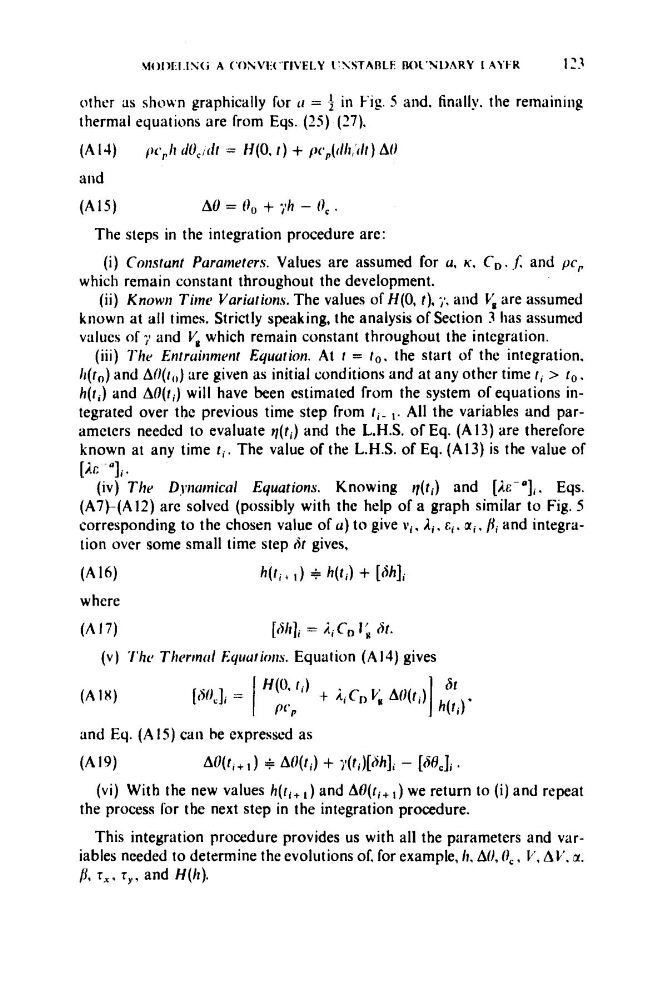
(v) ‘I‘lw Thc~rtnctl Equurioirs. Equation (A 14) gives
and Eq. (AIS) can be expressed as
(Al9)
AO(ti+ 1 ) + AO(ti) + y(fi)[Sh]i - [68,Ji I
(vi) With the new values h(ri+ and Atl(ri+ ,) we return to (i) and repeat
the process Tor the next step in the integration procedure.
This integration procedure provides us with all the parameters and variables needed to determine the evolutions of. for example, /I, AO, OE, V , AV. z.
/L 7, , T ~ ,
and H(lt).
thermal equations are from Eqs. (IS) (27).
(A 14)
/)<’,,/I dU,idt = H ( 0 . t ) + p~,,(d/i,’dt) A0
and
(A151
A0 = 0” + yh - Oc .
The steps in the integration procedure are:
(i) Cortstunf Paranterers. Values are assumed for u. K , CD, .f. and pc,
which remain constant throughout the development.
(ii) Known Time Variutions. The values of If(0, t), 7. and V, are assumed
known at all times. Strictly speaking, the analysis of Section 3 has assumed
values of 7 and V, which remain constant throughout the intcgration.
(iii) 7% Entruitrmnrf Eyuurion. At r = l o . the start of the integration,
/ ( t o ) and AO(i,,) are given as initial conditions and at any othcr time ri > lo.
h(ti) and AO(ti) will have been estimated from the system of equations integrated over the previous time step from t i - 1. All the variables and parameters needed to evaluate q(ri) and the L.H.S. of Eq. (A13) are therefore
known at any time t i . The value of the L.H.S. of Eq. (A13) is the value of
(iv) Tlir D!*ticrtnicu/ Eyuurions. Knowing ,](ti) and [h-’Ii. Eqs.
(A7)-(A12) are solved (possibly with the help of a graph similar to Fig. S
corresponding to the chosen value of a ) to give \Ii, di , ti. a i , pi and integration over some small time step rit gives,
[A; qi.
(A161
( A 17)
h(fi., ,) = h ( l i ) + [&Ii
[611], = RiCD 1; 6r.
where
(v) ‘I‘lw Thc~rtnctl Equurioirs. Equation (A 14) gives
and Eq. (AIS) can be expressed as
(Al9)
AO(ti+ 1 ) + AO(ti) + y(fi)[Sh]i - [68,Ji I
(vi) With the new values h(ri+ and Atl(ri+ ,) we return to (i) and repeat
the process Tor the next step in the integration procedure.
This integration procedure provides us with all the parameters and variables needed to determine the evolutions of. for example, /I, AO, OE, V , AV. z.
/L 7, , T ~ ,
and H(lt).