

S1'1~ADY-S'I'ATF ST4RI.E Hot 'NIJARY L A M W
83
1
3
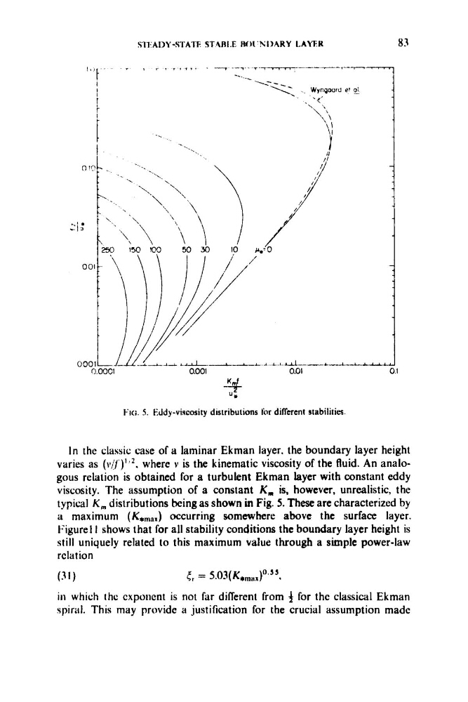
FIG. 5. Eddy-viscosity distributions Qr different stabilities
In the classic case of a laminar Ekman layer. the boundary layer height
varies as ( v / j ) I r 2 . where Y is the kinematic viscosity of the fluid. An analogous relation is obtained for a turbulent Ekman layer with constant eddy
viscosity. The assumption of a constant K, is, however, unrealistic, the
typical K, distributions being as shown in Fig. 5. These are characterized by
I maximum (K,,,,) occurring somewhere above the surface layer.
Figure1 I shows that for all stability conditions the boundary layer height is
still uniquely related to this maximum value through a simple power-law
rcla t ion
(31)
r, = 5.03(K*,,,)0.55,
in which thc cxponent is not far different from f for the classical Ekman
spiral. This may provide a justification for the crucial assumption made
83
1
3
FIG. 5. Eddy-viscosity distributions Qr different stabilities
In the classic case of a laminar Ekman layer. the boundary layer height
varies as ( v / j ) I r 2 . where Y is the kinematic viscosity of the fluid. An analogous relation is obtained for a turbulent Ekman layer with constant eddy
viscosity. The assumption of a constant K, is, however, unrealistic, the
typical K, distributions being as shown in Fig. 5. These are characterized by
I maximum (K,,,,) occurring somewhere above the surface layer.
Figure1 I shows that for all stability conditions the boundary layer height is
still uniquely related to this maximum value through a simple power-law
rcla t ion
(31)
r, = 5.03(K*,,,)0.55,
in which thc cxponent is not far different from f for the classical Ekman
spiral. This may provide a justification for the crucial assumption made