

10
Chapter 1: Toward an Ecological Geography of the Sea
production of ocean basins and smaller regions and already permit suggestive analysis
of decadal-scale trends in the global sea surface chlorophyll field; surface chlorophyll in
oligotrophic midocean gyres has significantly declined during the SeaWiFS era while over
some of the major shelf regions it has progressively increased (Gregg et al., 2003, 2005).
The analytical model that was used in the first ocean basin and global estimates of
oceanic primary production from satellite data required (i) surface chlorophyll, (ii) an
assumed photosynthesis/light relationship, (iii) surface irradiance, from sun angle and a
cloud cover climatology, and (iv) parameters descriptive of the chlorophyll profile. The
last item was obtained by reference to a global data base of 26,232 profiles each of which
was parameterized by its fit to a shifted Gaussian distribution, as described by Platt and
Sathyendranath (1988). This procedure delivered a unique definition of the shape of each
profile: the depth of the chlorophyll maximum, the standard deviation around the peak
value, the total pigment within the peak, the ratio of peak height to total pigment, and a
background chlorophyll value. Specifying that a minimum of six depths were required for
a successful fit of the model, 21,872 sets of profile parameters were used in a partitioned
global estimate of autotrophic production in the sea (Longhurst et al., 1995).
More recently, semiempirical methods have been developed that compute the same
rate from the surface chlorophyll field using a global equation that estimates the form of
the chlorophyll profile by means of an irradiance-independent, vertically integrated model
(e.g., Morel and Berthon, 1989). Semianalytical models, including that of Behrenfeld
and Falkowski (1997b), are routinely used by NASA at the Goddard Space Flight Center
to deliver global ocean production indices, binned weekly, monthly, and annually. An
image-based method has been devised for separating production fuelled by nitrate from
what is fuelled by regenerated ammonium and urea, a vital distinction in biological
oceanography (Sathyendranath et al., 1991).
The seasonal cycles of chlorophyll biomass and primary production for each province
that illustrate this book, from SeaWiFS sensors, were computed by George White with
a version of the Platt and Sathyendranath analytical model. Because some uncertainty
remains concerning the specification of photic depth from satellite images, integrated
pigment (Chl mg m
−2 ) was derived from the relationships obtained by Morel and Berthon
(1989) from a global set of chlorophyll profiles:
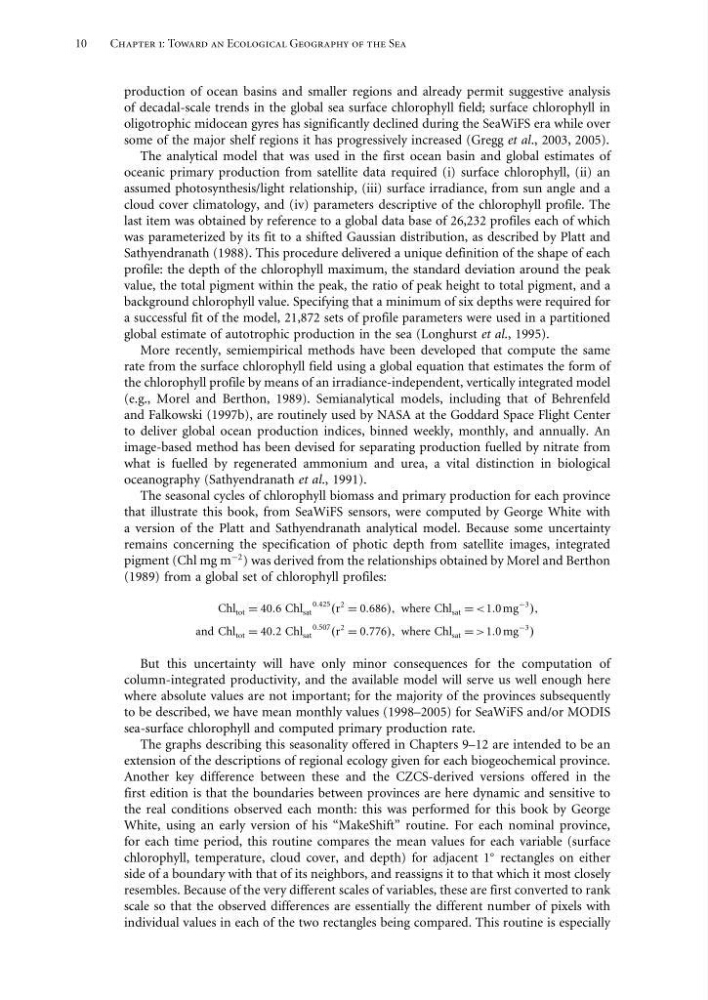
Chl tot = 406 Chl sat
0425 r
2 = 0686 where Chl sat = <10 mg
−3
and Chl tot = 402 Chl sat
0507 r
2 = 0776 where Chl sat = >10 mg
−3
But this uncertainty will have only minor consequences for the computation of
column-integrated productivity, and the available model will serve us well enough here
where absolute values are not important; for the majority of the provinces subsequently
to be described, we have mean monthly values (1998–2005) for SeaWiFS and/or MODIS
sea-surface chlorophyll and computed primary production rate.
The graphs describing this seasonality offered in Chapters 9–12 are intended to be an
extension of the descriptions of regional ecology given for each biogeochemical province.
Another key difference between these and the CZCS-derived versions offered in the
first edition is that the boundaries between provinces are here dynamic and sensitive to
the real conditions observed each month: this was performed for this book by George
White, using an early version of his “MakeShift” routine. For each nominal province,
for each time period, this routine compares the mean values for each variable (surface
chlorophyll, temperature, cloud cover, and depth) for adjacent 1
rectangles on either
side of a boundary with that of its neighbors, and reassigns it to that which it most closely
resembles. Because of the very different scales of variables, these are first converted to rank
scale so that the observed differences are essentially the different number of pixels with
individual values in each of the two rectangles being compared. This routine is especially
Chapter 1: Toward an Ecological Geography of the Sea
production of ocean basins and smaller regions and already permit suggestive analysis
of decadal-scale trends in the global sea surface chlorophyll field; surface chlorophyll in
oligotrophic midocean gyres has significantly declined during the SeaWiFS era while over
some of the major shelf regions it has progressively increased (Gregg et al., 2003, 2005).
The analytical model that was used in the first ocean basin and global estimates of
oceanic primary production from satellite data required (i) surface chlorophyll, (ii) an
assumed photosynthesis/light relationship, (iii) surface irradiance, from sun angle and a
cloud cover climatology, and (iv) parameters descriptive of the chlorophyll profile. The
last item was obtained by reference to a global data base of 26,232 profiles each of which
was parameterized by its fit to a shifted Gaussian distribution, as described by Platt and
Sathyendranath (1988). This procedure delivered a unique definition of the shape of each
profile: the depth of the chlorophyll maximum, the standard deviation around the peak
value, the total pigment within the peak, the ratio of peak height to total pigment, and a
background chlorophyll value. Specifying that a minimum of six depths were required for
a successful fit of the model, 21,872 sets of profile parameters were used in a partitioned
global estimate of autotrophic production in the sea (Longhurst et al., 1995).
More recently, semiempirical methods have been developed that compute the same
rate from the surface chlorophyll field using a global equation that estimates the form of
the chlorophyll profile by means of an irradiance-independent, vertically integrated model
(e.g., Morel and Berthon, 1989). Semianalytical models, including that of Behrenfeld
and Falkowski (1997b), are routinely used by NASA at the Goddard Space Flight Center
to deliver global ocean production indices, binned weekly, monthly, and annually. An
image-based method has been devised for separating production fuelled by nitrate from
what is fuelled by regenerated ammonium and urea, a vital distinction in biological
oceanography (Sathyendranath et al., 1991).
The seasonal cycles of chlorophyll biomass and primary production for each province
that illustrate this book, from SeaWiFS sensors, were computed by George White with
a version of the Platt and Sathyendranath analytical model. Because some uncertainty
remains concerning the specification of photic depth from satellite images, integrated
pigment (Chl mg m
−2 ) was derived from the relationships obtained by Morel and Berthon
(1989) from a global set of chlorophyll profiles:
Chl tot = 406 Chl sat
0425 r
2 = 0686 where Chl sat = <10 mg
−3
and Chl tot = 402 Chl sat
0507 r
2 = 0776 where Chl sat = >10 mg
−3
But this uncertainty will have only minor consequences for the computation of
column-integrated productivity, and the available model will serve us well enough here
where absolute values are not important; for the majority of the provinces subsequently
to be described, we have mean monthly values (1998–2005) for SeaWiFS and/or MODIS
sea-surface chlorophyll and computed primary production rate.
The graphs describing this seasonality offered in Chapters 9–12 are intended to be an
extension of the descriptions of regional ecology given for each biogeochemical province.
Another key difference between these and the CZCS-derived versions offered in the
first edition is that the boundaries between provinces are here dynamic and sensitive to
the real conditions observed each month: this was performed for this book by George
White, using an early version of his “MakeShift” routine. For each nominal province,
for each time period, this routine compares the mean values for each variable (surface
chlorophyll, temperature, cloud cover, and depth) for adjacent 1
rectangles on either
side of a boundary with that of its neighbors, and reassigns it to that which it most closely
resembles. Because of the very different scales of variables, these are first converted to rank
scale so that the observed differences are essentially the different number of pixels with
individual values in each of the two rectangles being compared. This routine is especially